Gradient descent
The goal of this chapter is to provide a quick overview of gradient descent based optimization and how it interacts with deep source separation models. Gradient descent is how nearly all modern deep nets are trained. Many more in-depth resources exist out there, as this chapter will only scratch the surface. The learning outcomes of this chapter are:
Understand at a high-level what gradient descent is doing and how it works.
Understand and be able to choose between different optimization algorithms.
Be able to investigate various aspects of the learning process for debugging, diagnosing issues in your training scripts, or intellectual curiosity.
First, let’s set up a simple example through which we can investigate gradient descent. Let’s learn a simple linear regression. There are more straightforward ways to learn linear regression, but for the sake of pedagogy, we’ll start with this simple problem. We’ll use PyTorch as our ML library for this.
%%capture
!pip install scaper
!pip install nussl
!pip install git+https://github.com/source-separation/tutorial
import torch
from torch import nn
import nussl
import numpy as np
import matplotlib.pyplot as plt
import gif
from IPython.display import display, Image
import tempfile
import copy
import tqdm

nussl.utils.seed(0)
to_numpy = lambda x: x.detach().numpy()
to_tensor = lambda x: torch.from_numpy(x).reshape(-1, 1).float()

def show_gif(frames, duration=5.0, width=600):
    with tempfile.NamedTemporaryFile(suffix='.gif') as f:
        gif.save(frames, f.name, duration=duration)
        with open(f.name,'rb') as f:
            im = Image(data=f.read(), format='png', width=width)
    return im
Introduction
Let’s make a single layer neural network with 1 hidden unit. This is just a line, and corresponds to:
where \(y\) is the output of the network, and \(m\) and \(b\) are learnable parameters.
class Line(nn.Module):
    def __init__(self):
        super().__init__()
        self.layer = nn.Linear(1, 1)

    def forward(self, x):
        y = self.layer(x)
        return y

line = Line()
x = torch.randn(100, 1)
y = line(x)

plt.title("Prediction of network at iteration. 0")
plt.scatter(to_numpy(x), to_numpy(y))
plt.show()
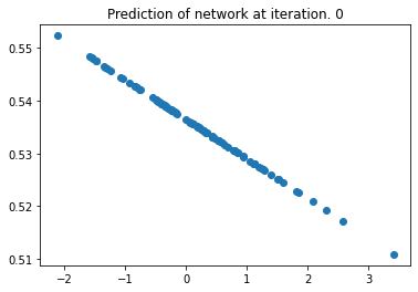
The network is randomly initialized, and we passed some random data through it.
Since it’s a single linear layer with one unit, we can see that it is a line.
The magic is hidden away inside the nn.Linear call. PyTorch initializes
a single network layer with one hidden unit (\(m\)) and a bias (\(b\)):
for n, p in line.named_parameters():
    print(n, p)
layer.weight Parameter containing:
tensor([[-0.0075]], requires_grad=True)
layer.bias Parameter containing:
tensor([0.5364], requires_grad=True)
layer.weight corresponds to \(m\) and layer.bias corresponds to \(b\). Note
the way we are iterating over the parameters in the network - that’ll be
important later on!
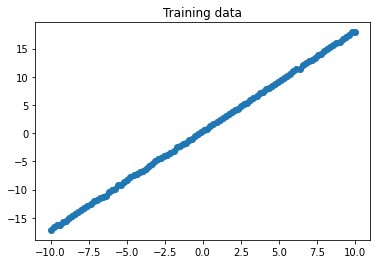
Now that we’ve got our simple model, let’s make some training data. The training data here will be a line of some slope with some bias, plus a bit of random noise with a mean of \(0\) and standard deviation \(\sigma\). In math, it’s like this:
We will try to recover \(m\) and \(b\) as close as possible via gradient descent. Okay, let’s make the data:
m = np.random.randn()
b = np.random.randn()
x = np.linspace(-10, 10, 100)
noise = np.random.normal(loc=0, scale=0.1, size=100)

y = m*x + b + noise

plt.title("Training data")
plt.scatter(x, y)
plt.show()
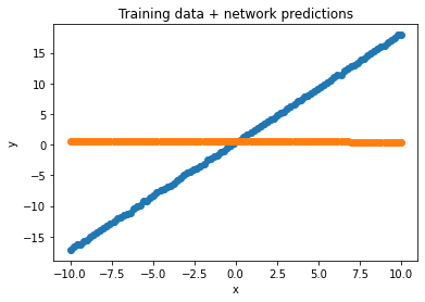
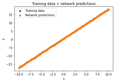
Let’s look at what our network does on this data, overlaid with the actual training data:
y_hat = line(to_tensor(x))

plt.title("Training data + network predictions")
plt.scatter(x, y, label='Training data')
plt.scatter(x, to_numpy(y_hat), label='Network predictions')
plt.xlabel('x')
plt.ylabel('y')
plt.show()
Loss functions
Let’s now take a look at how gradient descent can be used to learn \(m\) and \(b\) directly from the training data. The first thing we need is a way to tell how well the network is doing right now. That is to say, how accurate are its predictions? To do this, we need a loss function. A very simple one would just be to take the absolute difference between the predictions and the ground truth:
where \(\theta\) is our neural network function, which does the following operation:
where \(\hat{m}\) and \(\hat{b}\) are the current parameters of the network.
So, how’s our network doing?
loss = (y_hat - to_tensor(y)).abs()
plt.title("Loss for each data point")
plt.scatter(x, to_numpy(loss))
plt.ylabel("Loss")
plt.xlabel("x")
plt.show()
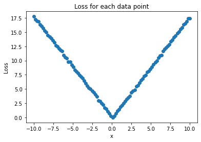
Above you can see the loss for every point in our training data. But in order to do the next step, we will need to represent the performance of the network as a single number. To do this, we’ll just take the mean:
loss.mean()
tensor(8.9430, grad_fn=<MeanBackward0>)
Why the mean and not the sum or some other aggregator? Well, the mean is nice because it stays in the same range no matter how many data points you compute the loss over, unlike the sum. Second, we want to increase the performance across the board, so we wouldn’t want to use max or some operation that only looks at one data point.
Brute-force approach
Now that we’ve got a measure of how well our network is doing, how do we make the network better? The goal is to reduce the loss. Let’s do this in a really naive way first: let’s guess! We’ll do a search over all the possible network parameters for our Line module within some range, and compute the loss for each one:
possible_m = np.linspace(-2, 2, 100)
possible_b = np.linspace(-2, 2, 100)
loss = np.empty((
    possible_m.shape[0],
    possible_b.shape[0]
))

with torch.no_grad():
    for i, m_hat in enumerate(possible_m):
        for j, b_hat in enumerate(possible_b):
            line.layer.weight[0, 0] = m_hat
            line.layer.bias[0] = b_hat
            y_hat = line(to_tensor(x))
            _loss = (y_hat - to_tensor(y)).abs().mean()
            loss[i, j] = _loss

plt.title('2D Visualization of Loss Landscape')
plt.pcolormesh(possible_m, possible_b, loss, shading='auto')
plt.colorbar()
plt.xlabel('Value of m')
plt.ylabel('Value of b')
plt.show()
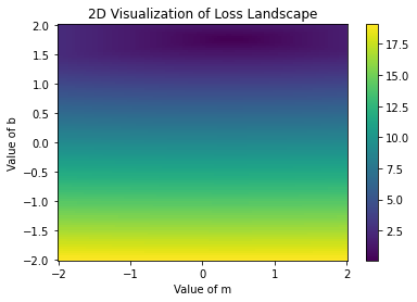
What we did: iterate over all values of \(m\) and \(b\) above and compute the loss. Then, we plotted the loss in a 2D visualization. We can see the dark blue part of the image, which indicates where the loss is minimized. Let’s see what the actual value is:
idx = np.unravel_index(np.argmin(loss, axis=None), loss.shape)
m_hat = possible_m[idx[0]]
b_hat = possible_b[idx[1]]

print(f"Loss minimum of {loss.min():-2f} at \n\t m_hat={m_hat:0.2f}, b_hat={b_hat:-.2f}")
print(f"Actual m, b: \n\t m={m:.2f}, b={b:.2f}")
Loss minimum of 0.086866 at
	 m_hat=1.76, b_hat=0.38
Actual m, b:
	 m=1.76, b=0.40
Here’s what the network predictions look like, with the learned line:
with torch.no_grad():
    line.layer.weight[0, 0] = m_hat
    line.layer.bias[0] = b_hat

    y_hat = line(to_tensor(x))

plt.title("Training data + network predictions")
plt.scatter(x, y, label='Training data')
plt.scatter(x, to_numpy(y_hat), label='Network predictions')
plt.xlabel('x')
plt.ylabel('y')
plt.legend()
plt.show()
Iterating over all possible \(m\) and \(b\) values in a range worked here, but it’s not a great thing in general. We only have \(2\) parameters here, and we did \(100\) choices for each, so that worked out to \(100 * 100\) = 10k “iterations” to learn a line! How do we cut this down? By using gradient descent, of course.
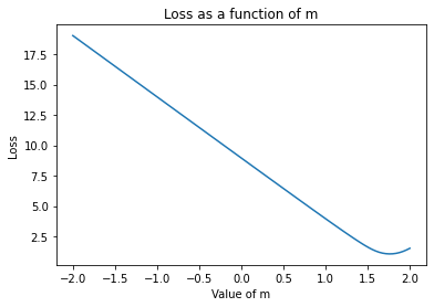
Gradient descent
In gradient descent, we look at the local loss landscape - where we are now and the points that we could go to around us. To make things simpler, let’s use the data we generated above to look at how the loss changes as the value of \(m\) changes:
plt.plot(possible_m, loss.mean(axis=1))
plt.xlabel('Value of m')
plt.ylabel('Loss')
plt.title('Loss as a function of m')
plt.show()
Now, let’s look at it as \(b\) changes:
plt.plot(possible_b, loss.mean(axis=0))
plt.xlabel('Value of b')
plt.ylabel('Loss')
plt.title('Loss as a function of b')
plt.show()
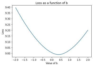
The slope of these curves is the gradient. For example, in the first \(m\) plot, we see the loss goes down as \(m\) increases from \(-1\) to \(-.75\) roughly linearly. The gradient between these points is simply the change in the loss with respect to \(m\) as you change it from \(-1\) to \(-.75\): about \(-1\). By using the gradient to continue in the direction that makes the loss go down, we are doing gradient descent. Note that at the minima - where the loss is lowest, the gradient is \(0\).
PyTorch has an easy way of computing gradients: the backward() function. To compute
the gradients, just compute the loss and then call backward() on it.
line = Line()
with torch.no_grad():
    line.layer.weight[0, 0] = m_hat
    line.layer.bias[0] = b_hat

y_hat = line(to_tensor(x))
_loss = (y_hat - to_tensor(y)).abs().mean()
_loss.backward()

line.layer.weight.grad, line.layer.bias.grad
(tensor([[-0.8747]]), tensor([-0.1000]))
So the weight has a gradient flowing through it, as does the bias. Let’s do the same thing we did for the loss before, but this time let’s look at the gradients as \(m\) and \(b\) change:
possible_m = np.linspace(-1, 1, 100)
possible_b = np.linspace(-1, 1, 100)
grad_m = np.empty((
    possible_m.shape[0],
    possible_b.shape[0]
))
grad_b = np.empty((
    possible_m.shape[0],
    possible_b.shape[0]
))

for i, m_hat in enumerate(possible_m):
    for j, b_hat in enumerate(possible_b):
        line = Line()
        with torch.no_grad():
            line.layer.weight[0, 0] = m_hat
            line.layer.bias[0] = b_hat
        y_hat = line(to_tensor(x))
        _loss = (y_hat - to_tensor(y)).abs().mean()
        _loss.backward()

        grad_m[i, j] = line.layer.weight.grad.item()
        grad_b[i, j] = line.layer.bias.grad.item()

plt.plot(possible_m, grad_m.mean(axis=1))
plt.xlabel('Value of m')
plt.ylabel('Gradient')
plt.title('Gradient as a function of m')
plt.show()

plt.plot(possible_b, grad_b.mean(axis=1))
plt.xlabel('Value of b')
plt.ylabel('Gradient')
plt.title('Gradient as a function of b')
plt.show()
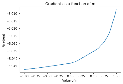
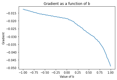
Above we can see that at each value of \(m\) or \(b\) the gradient tells us which way will increase the loss. Below the optimal value of \(\hat{m}\), it’s telling us that decreasing \(\hat{m}\) will increase the loss. So therefore, we must go in the opposite direction of the gradient. Let’s put it all together:
Compute the gradient for the current network parameters \(\hat{m}\) and \(\hat{b}\).
Go in the opposite direction of the gradient by some fixed amount.
Go back to 1.
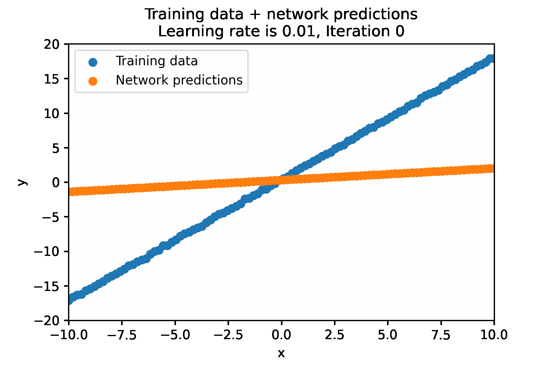
In a simple for loop, it looks like this:
N_ITER=100
LEARNING_RATE = 0.01
# initialize line
line = Line()

frames = []
@gif.frame
def plot(i):
    y_hat = line(to_tensor(x))
    plt.figure(dpi=300)
    plt.title(
        f"Training data + network predictions\n"
        f"Learning rate is {LEARNING_RATE}, Iteration {i}")

    plt.scatter(x, y, label='Training data')
    plt.scatter(x, to_numpy(y_hat), label='Network predictions')
    plt.xlabel('x')
    plt.ylabel('y')
    plt.xlim([-10, 10])
    plt.ylim([-20, 20])
    plt.legend()

for i in range(N_ITER):
    line.zero_grad()
    y_hat = line(to_tensor(x))
    _loss = (y_hat - to_tensor(y)).abs().mean()
    _loss.backward()

    for n, p in line.named_parameters():
        p.data += - LEARNING_RATE * p.grad

    frame = plot(i)
    frames.append(frame)

show_gif(frames)
Impact of learning rate
The key hyperparameter to consider here is the learning rate. The learning rate controls how big of a step you take in the direction away from the gradient. Let’s see how this parameter can affect the performance of gradient descent, by trying a few different values, and visualizing the learning process for each one:
N_ITER=100
LEARNING_RATES = [1.0, 0.5, 0.1, 0.01, 0.001, 0.0001]

line = Line()
lines = [copy.deepcopy(line) for _ in LEARNING_RATES]

losses = [[] for _ in range(len(LEARNING_RATES))]
grad_norms = [[] for _ in range(len(LEARNING_RATES))]

frames = []
@gif.frame
def plot(i, lines):
    ncols = 3
    nrows = len(LEARNING_RATES) // ncols
    width = ncols * 5
    height = nrows * 4
    fig, axs = plt.subplots(nrows, ncols, dpi=100, figsize=(width, height))
    axs = axs.flatten()

    for j, line in enumerate(lines):
        y_hat = line(to_tensor(x))
        axs[j].set_title(
            f"Training data + network predictions\n"
            f"Learning rate is {LEARNING_RATES[j]}, Iteration {i}")
        axs[j].scatter(x, y, label='Training data')
        axs[j].scatter(x, to_numpy(y_hat), label='Network predictions')
        axs[j].set_xlabel('x')
        axs[j].set_ylabel('y')
        axs[j].legend()
        axs[j].set_xlim([-10, 10])
        axs[j].set_ylim([-20, 20])

    plt.tight_layout()

for i in range(N_ITER):
    for j, line in enumerate(lines):
        line.zero_grad()
        y_hat = line(to_tensor(x))
        _loss = (y_hat - to_tensor(y)).abs().mean()
        losses[j].append(_loss)
        _loss.backward()

        grad_norm = 0
        for n, p in line.named_parameters():
            p.data += - LEARNING_RATES[j] * p.grad
            grad_norm += (p.grad.sum() ** 2)
        grad_norm = grad_norm.sqrt().item()
        grad_norms[j].append(grad_norm)

    frame = plot(i, lines)
    frames.append(frame)

show_gif(frames, width=1200)
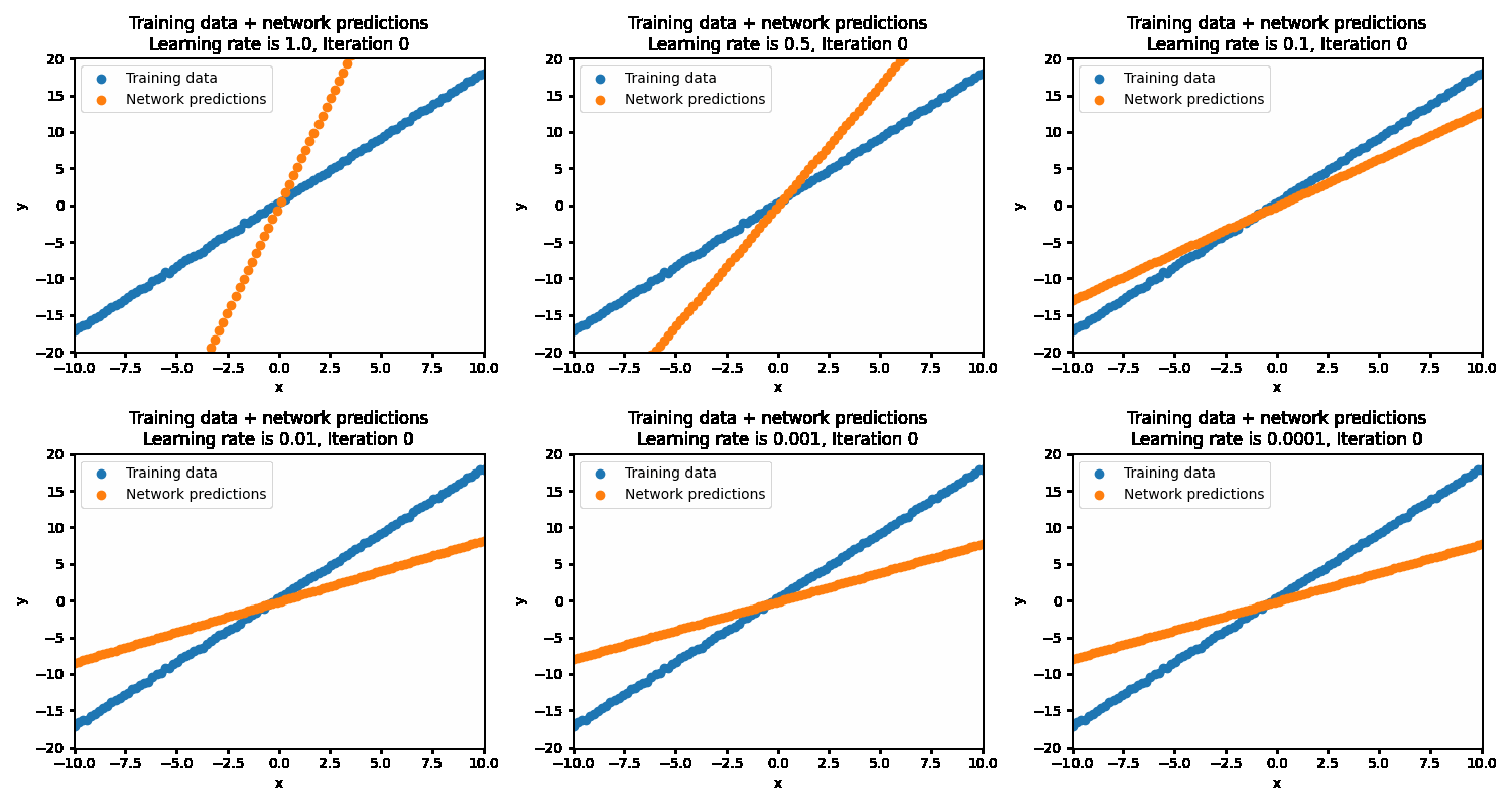
If the learning rate is set too high, then the correct solution is never reached as the steps being taken are much too large. This results in the optimization oscillating back and forth between different parameters. At the more optimal learning rate of 0.01, the optimizations succeeds in finding the best parameters. At too low of a learning rate (0.001 and below), the optimization will eventually reach the optimal point but will be very inefficient in getting there.
With the optimal learning rate, our model learns the true data distribution within 25 iterations. Much more efficient than the 10k iterations for brute forcing!
Tip
You’ll always want your learning rate to be set as high as possible, but not so high that optimization becomes unstable. Lower learning rates are generally “safer” in terms of reaching minima, but are more inefficient. Soon, we’ll look at ways that you can monitor the health of your training procedure and how that help guide your choices for optimization hyperparameters.
Signs of healthy training
The network that we’ve looked at so far is an exceedingly simple one. Deep audio models are of course not single one-weight layer networks. Much of the analysis that we’ve done so far is not possible in high dimensions. There are essentially two core tools that one can use to diagnose and monitor network training:
The training and validation loss
The gradient norm
By monitoring these two metrics, one can get a good idea of whether the learning rate is set too high or too low, whether different optimization algorithms should be used, etc.
Let’s examine the behavior of these for each of the 6 learning rates above. In that code, we saved the loss history as well as the norm of the gradient at each iteration.
fig, ax = plt.subplots(1, 2, figsize=(15, 5))

for j, lr in enumerate(LEARNING_RATES):
    ax[0].plot(grad_norms[j], label=f'Learning rate: {lr}')
    ax[0].legend()
    ax[0].set_xlabel('Iteration')
    ax[0].set_ylabel('grad norm')
    ax[0].set_title('Gradient norm for each learning rate')

for j, lr in enumerate(LEARNING_RATES):
    ax[1].plot(np.log10(losses[j]), label=f'Learning rate: {lr}')
    ax[1].legend()
    ax[1].set_xlabel('Iteration')
    ax[1].set_ylabel('log(loss)')
    ax[1].set_title('Loss for each learning rate')
plt.show()
---------------------------------------------------------------------------
RuntimeError                              Traceback (most recent call last)
<ipython-input-18-91a4bf5517c3> in <module>
      9
     10 for j, lr in enumerate(LEARNING_RATES):
---> 11     ax[1].plot(np.log10(losses[j]), label=f'Learning rate: {lr}')
     12     ax[1].legend()
     13     ax[1].set_xlabel('Iteration')

/opt/hostedtoolcache/Python/3.7.10/x64/lib/python3.7/site-packages/torch/tensor.py in __array__(self, dtype)
    619             return handle_torch_function(Tensor.__array__, (self,), self, dtype=dtype)
    620         if dtype is None:
--> 621             return self.numpy()
    622         else:
    623             return self.numpy().astype(dtype, copy=False)

RuntimeError: Can't call numpy() on Tensor that requires grad. Use tensor.detach().numpy() instead.
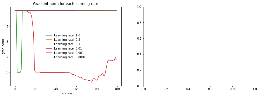
How do we interpret these plots? The plot on the right tells us that for some learning rates, we get an oscillating behavior in the loss, suggesting we are jumping rapidly from very different points in the space. The plot on the left suggests that we start from a place that has very high gradient norm. Because of this, combined with the high learning rate, we get this oscillating behavior. The optimal learning rate starts with high gradient norm, but as it moves closer to the minima, the gradient norm decreases, indicating healthy training.
Tip
When training your own networks, even big ones, it can be really helpful to look at these plots and adjust your hyperparameters accordingly.
Note
There is extensive research into better optimization procedures. Here we are looking at SGD (Stochastic Gradient Descent), but in practice we will use a momentum-based optimizer.
Enough rambling - what do i use?!
In any deep learning project, it’s easy to get bogged down in “hyperparameter hell”, where the loss landscape is spikey, scary, and full of nightmares. Sometimes, it seems that no matter what you do, the loss simply won’t go down, or it won’t reach the loss reported in paper X, etc. We’ve all been there. In this section, the goal is to introduce the most common settings that are in a lot of different source separation papers.
Optimizer choice
The choice of optimizer is most often the ADAM optimizer. ADAM is an optimizer which traverses the loss landscape using momentum. If you’re new to momentum, here’s a fantastic resource to get acquainted with it: https://distill.pub/2017/momentum/.
In momentum-based optimization, the idea is to adaptively change the learning rate based on the history of the gradients. If gradients are small, but they’re always pointing in the same direction as you traverse the loss landscape, that indicates that you can take bigger steps! Bigger steps means more efficient learning. ADAM codifies this logic via some math that we don’t have to get into here. It suffices to understand that the idea of ADAM is that more consistent gradients leads to faster learning. To quote the Distill post above - if gradient descent is a person walking down a hill, then momentum is a ball rolling down a hill. The ball picks up speed as it rolls.
Momentum-based optimization is a very common choice in the source separation literature. Specifically, ADAM is used with the following hyperparameters being a good initial setup (that you likely won’t have to change):
ADAM Optimizer
Learning rate: 1e-3
\(\beta_1\) = .9, \(\beta_2\) = .999
Lucky for you, these are the PyTorch defaults (funny how that works)!
Gradient clipping
Another popular trick to improve optimization is to use gradient clipping. In many loss landscapes, the gradient is not perfectly smooth as we have seen so far. Often, the loss landscape is exceedingly noisy, with many small bumps and imperfections. These imperfections can lead to huge spikes in the gradient, which can destabilize the learning process.
The damage that huge spikes in the loss landscape can do to optimization can be mitigated via gradient clipping. Simply put, in gradient clipping if the gradient norm exceeds some set threshold, then it is renormalized such that the norm of the gradient is equal to that threshold. If the norm is below the set threshold, then the gradient is untouched.
Why does gradient clipping work so well, theoretically? Well, it’s a bit of an open question right now with a long history [BSF94,Mik12], and a lot of interesting recent work [ZHSJ19]!
Tip
Exploding gradients, along with vanishing gradients are important to look out for. Note that most recurrent network architectures are susceptible to both types of gradient issues, and that the best way to stabilize training and overcome exploding gradients is via gradient clipping. Gradient clipping is an important part of the recipe for many state-of-the-art separation networks.
AutoClip
Picking the optimal gradient clipping threshold can be tough, and choosing it poorly can lead to bad results. Recent work [SWPR20] proposes an automated mechanism to choose the gradient clipping threshold by using the history of the gradient norms in conjunction with a simple percentile based approach. For more, see here (full disclosure: the author of this method is currently writing what you’re reading now).
In summary, use the Adam optimizer combined with some flavor of gradient clipping (either with a hand-tuned threshold, or with AutoClip) to train your network. In the next section, we’ll start to explore actual models, their building blocks, and how things are put together.