Coding up model architectures¶

Most deep separation networks that have cropped up in recent years use and re-use many of the same components. While some papers introduce new types of layers, often there are still components that can be abstracted out and used across multiple network architectures. This structure has solidified in recent years, with at least two open source projects - Asteroid and nussl - recognizing this.

This chapter is meant to acquaint you with the exact implementations of each of these building blocks, and eventually build them up to a few different, interesting, network architectures that are seen throughout the source separation literature.

%%capture
!pip install scaper
!pip install nussl
!pip install git+https://github.com/source-separation/tutorial

Deep mask estimation¶

Our story starts with one of the more established methods for deep audio source separation - learning the mask. Recall that the goal of many audio source separation algorithms before deep learning was to construct the optimal mask that when applied to the STFT (or other invertible time-frequency representation such as the CQT) of the mixture, produced an estimate of the isolated source - vocals, accompaniment, speaker one, speaker two, etc. When deep networks first came on the scene, one obvious thing to do was to create a deep network that would predict the masks directly.

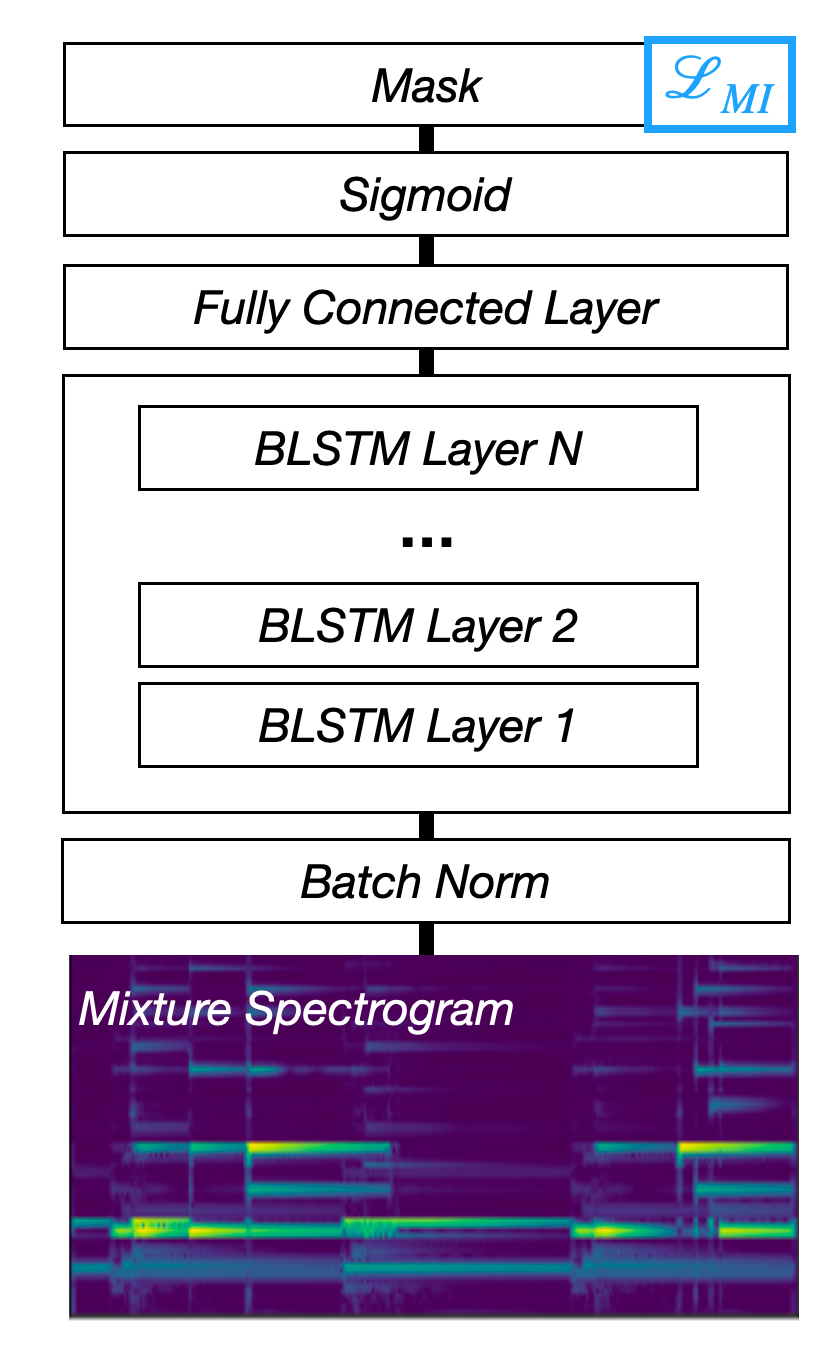
Fig. 49 A diagram of the Mask Inference architecture.¶

Note

Some early work tried to predict the magnitudes directly, but this generally resulted in worse performance. Things may be changing though, with some recent work.

Model overview¶

In the sections below we will be building up a deep mask estimation model. The model takes a representation of the mixture (the magnitude spectrogram), and converts it into a mask with the following steps:

Convert magnitude spectrogram to log-magnitude spectrogram.
Normalize the log-magnitude spectrogram.
Process the log-magnitude spectrogram with a stack of recurrent neural networks.
Convert the output of the recurrent stack to a mask that can be applied to the mixture.

This is a “simple” model that is for mostly pedagogical purposes, but does work well for some separation problems. We’ll look at more complicated models later on.

We’ll start with the last step, so that we understand the output of the network. Then, we’ll learn how to do the first 3 steps. A model in PyTorch always looks like this:

import torch
from torch import nn
import nussl

nussl.utils.seed(0)
to_numpy = lambda x: x.detach().numpy()
to_tensor = lambda x: torch.from_numpy(x).reshape(-1, 1).float()

class Model(nn.Module):
    def __init__(self):
        super().__init__()
    
    def forward(self, data):
        return data

In the __init__ function, you save everything the model needs to do its computation. This includes initialized building blocks, and any other variables needed. In the forward function, you define the actual data flow of the model as it goes from input to output (in this case a mask).

Masking¶

The first building block we’ll look at is one of the simplest ones - a mask. As we saw in previous chapters, one way to perform separation is to element-wise multiply a mask with a representation. This representation is generally the magnitude spectrogram. We’ll start by introducing it in numpy, and then move towards doing it in PyTorch.

import torch
import nussl
from common import viz
import numpy as np
import matplotlib.pyplot as plt

musdb = nussl.datasets.MUSDB18(download=True)
item = musdb[40]

viz.show_sources(item['sources'])

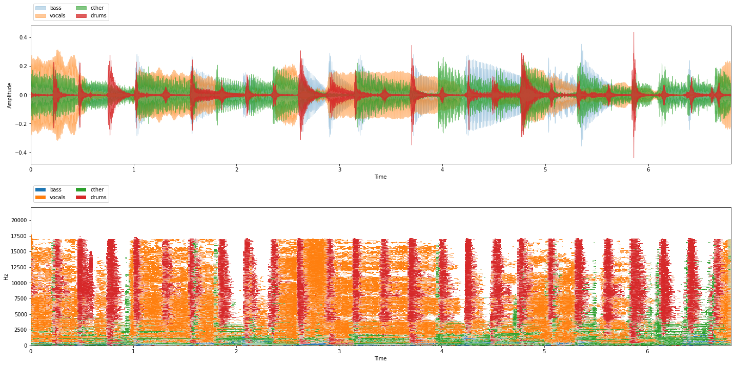
In the lower plot, we can see a visualization of the mask required for each source to separate it from the mixture. Let’s do the operation of actually masking in numpy first:

representation = np.abs(item['mix'].stft())
vocals_representation = np.abs(item['sources']['vocals'].stft())

fig, ax = plt.subplots(1, 2, figsize=(15, 4))
ax[0].imshow(20 * np.log10(representation[..., 0]), origin='lower', aspect='auto')
ax[0].set_title('Mixture spectrogram')
ax[1].imshow(20 * np.log10(vocals_representation[..., 0]), origin='lower', aspect='auto')
ax[1].set_title('Vocals spectrogram')
plt.show()

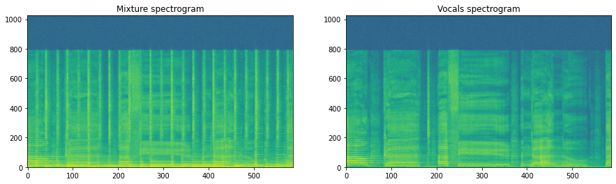
Now that we’ve got the representation of both the mixture spectrogram and the vocals spectrogram, let’s build a soft mask for the vocals. This is done via the following formula, where mask \(\hat{M}(t, f) \in [0, 1]\), \(Y(t, f)\) is the energy of the mixture spectrogram at each time-frequency point, and \(S_i(t, f)\) is the energy of the vocals spectrogram at each time-frequency point:

\[S_i(t, f) = \hat{M}(t, f) * Y(t, f)\]

We can solve for \(\hat{M}\):

\[\frac{S_i(t, f)}{\max(S_i(t, f), Y(t, f)) + \epsilon} = \hat{M}(t, f) \]

We take the maximum of the source spectrogram and the mixture spectrogram so that \(\hat{M}(t, f)\) stays between \(0\) and \(1\). This will become important later when we actually build the network. Okay, so given all that, the implementation is straightforward in numpy:

mask = vocals_representation / (np.maximum(vocals_representation, representation) + 1e-8)

fig, ax = plt.subplots(1, 2, figsize=(15, 4))
ax[0].imshow(20 * np.log10(representation[..., 0]), origin='lower', aspect='auto')
ax[0].set_title('Mixture spectrogram')
ax[1].imshow(mask[..., 0], origin='lower', aspect='auto')
ax[1].set_title('Vocals mask')
plt.show()

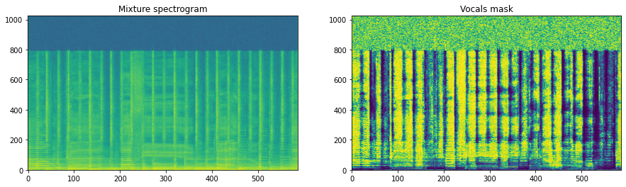
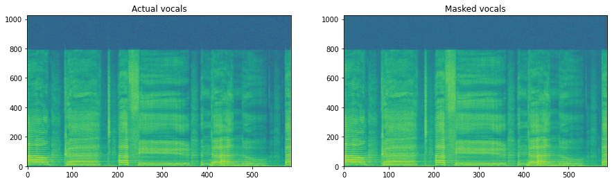
Now we see the actual mask. To actually apply the mask, just multiply it element-wise with the mixture spectrogram:

masked = mask * representation
fig, ax = plt.subplots(1, 2, figsize=(15, 4))
ax[0].imshow(20 * np.log10(vocals_representation[..., 0]), origin='lower', aspect='auto')
ax[0].set_title('Actual vocals')
ax[1].imshow(20 * np.log10(masked[..., 0]), origin='lower', aspect='auto')
ax[1].set_title('Masked vocals')
plt.show()

Let’s actually listen to the separation by combining the masked magnitudes with the mixture phase:

mix_phase = np.angle(item['mix'].stft())
masked_stft = masked * np.exp(1j * mix_phase)
new_signal = nussl.AudioSignal(stft=masked_stft, sample_rate=item['mix'].sample_rate)
new_signal.istft()
new_signal.embed_audio(display=False)

Sounds pretty good! We’ve established that masking works pretty well for separating sources, and that masking is a relatively easy operation. Let’s convert things to PyTorch tensors to see how the numpy code above translates:

mix_tensor = torch.from_numpy(representation)
mask_tensor = torch.rand_like(mix_tensor.unsqueeze(-1))

# shapes
print(mix_tensor.shape, mask_tensor.shape)

# masking operation:
masked_tensor = mix_tensor.unsqueeze(-1) * mask_tensor

print(masked_tensor.shape)

torch.Size([1025, 587, 2]) torch.Size([1025, 587, 2, 1])
torch.Size([1025, 587, 2, 1])

Here, we just constructed a random mask and then element-wise multiplied it. One thing to note here are the shapes! The shape of the mix tensor is:

Number of frequency bins in FFT
Number of time steps
Number of audio channels

The mask tensor has one additional dimension:

Number of sources (here only 1 source).

Note

In practice, there will also be a batch dimension, which will be the 0th dimension. Also, in general, the time dimension will be the first non-batch dimension (1st), and frequency will be the 2nd. This is a matter of convention, however. The important thing is to say consistent. In nussl, this is the convention that is expected from all building blocks.

So for example, to separate four sources, we would just need 4 masks that are stacked. When multiplied against the mix tensor, it broadcasts, resulting in 4 separated sources. Note that we needed to unsqueeze the mix tensor, adding an extra dummy dimension, so that this multiplication works.

The point of the rest of the blocks in this section is to create a mask that we can apply to the time-frequency representation of the mixture. Keep this in mind as we introduce the rest of the blocks. First, let’s introduce different ways we can process the mixture spectrogram.

Log-magnitude representation¶

One component of this model (but not all models) is to compute the log-magnitude representation. To see why we do this, compare the histogram of the magnitude-spectrogram with the log-magnitude spectrogram:

fig, ax = plt.subplots(1, 2, figsize=(15, 4))
ax[0].hist(20 * np.log10(np.maximum(representation, 1e-8)).flatten(), bins=50)
ax[0].set_title('Log-magnitude distribution')
ax[1].hist(representation.flatten(), bins=50)
ax[1].set_title('Magnitude distribution')
plt.show()

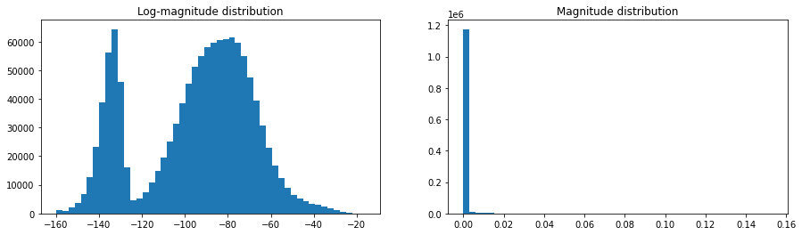
Distributions that look those on the left are generally more much friendly for neural network training. Second, log-magnitude representations more closely match the human perception of volume which is logarithmic, not linear. A 3dB boost in volume perceptually doubles the volume of a sound. Log-magnitude representations generally give neural networks a leg up, both in terms of activations as well as a good representation of the audio that it starts from.

To do this in nussl, we simply use the AmplitudeToDB layer that is built in:

from nussl.ml.networks.modules import AmplitudeToDB

amplitude_to_db = AmplitudeToDB()
mix_log_amplitude = amplitude_to_db(mix_tensor)
print(mix_tensor.mean(), mix_log_amplitude.mean())

tensor(0.0004, dtype=torch.float64) tensor(-75.9872, dtype=torch.float64)

Now let’s put this in our actual model as our first building block. Let’s also reshape the mix_tensor a bit for future use so that it follows this pattern (which is what nussl building blocks expect):

Dim 0: Batch size
Dim 1: Sequence length (# of time steps)
Dim 2: # of frequency bins
Dim 3: # of audio channels (not to be confused with convolutional channels)

mix_tensor.shape

torch.Size([1025, 587, 2])

print("Shape before (nf, nt, nac): ", mix_tensor.shape)
mix_tensor = mix_tensor.permute(1, 0, 2).unsqueeze(0).float()
print("Shape after (nb, nt, nf, nac):", mix_tensor.shape)

Shape before (nf, nt, nac):  torch.Size([1025, 587, 2])
Shape after (nb, nt, nf, nac): torch.Size([1, 587, 1025, 2])

class Model(nn.Module):
    def __init__(self):
        super().__init__()
        
        self.amplitude_to_db = AmplitudeToDB()
    
    def forward(self, data):
        data = self.amplitude_to_db(data)
        return data
    
model = Model()
mix_log_amplitude = model(mix_tensor)

Our model now takes a mix spectrogram and computes the log magnitude features.

Input normalization¶

Input normalization is a critical feature of most deep separation models. In neural networks, activation functions work best within a limited range of values. For example, let’s look at a plot of the Sigmoid activation function:

x = torch.linspace(-6, 6, 1000)
y = torch.sigmoid(x)
plt.plot(to_numpy(x), to_numpy(y))
plt.xlabel('x')
plt.ylabel('sigmoid(x)')
plt.title('Sigmoid activation function')
plt.show()

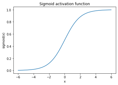
The “good” range for the Sigmoid function is between -6 and 6. What happens as you go further out?

x = torch.linspace(-100, 100, 1000)
y = torch.sigmoid(x)
plt.plot(to_numpy(x), to_numpy(y))
plt.xlabel('x')
plt.ylabel('sigmoid(x)')
plt.title('Sigmoid activation function')
plt.show()

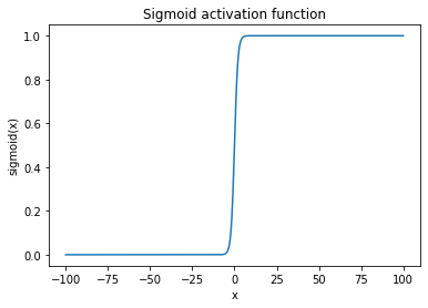
The sigmoid function saturates more and more below \(-6\) or above \(6\). This means that the activations coming from this layer will be basically useless if we feed in log-magnitude spectrogram features which range from \(-160\) to \(-20\). Not just Sigmoid, but all activation functions such as TanH, ReLU, etc. have this issue. So in order to give the network the best chance at learning what we want it to learn, we use input normalization. The same principles can apply to inner layers of the network as well (e.g. batch normalization, layer normalization, etc). The simplest way to apply input normalization (sometimes also called whitening), is to use nussl’s BatchNorm layer, as follows:

from nussl.ml.networks.modules import BatchNorm

def print_stats(data):
    print(
        f"Shape: {data.shape}\n"
        f"Mean: {data.mean().item()}\n"
        f"Var: {data.var().item()}\n"
    )

input_normalization = BatchNorm(num_features=mix_tensor.shape[2])
mix_log_amplitude = amplitude_to_db(mix_tensor)

print_stats(mix_tensor)
print_stats(mix_log_amplitude)

normalized = input_normalization(mix_log_amplitude)

print_stats(mix_log_amplitude)
print_stats(normalized)

Shape: torch.Size([1, 587, 1025, 2])
Mean: 0.00044009656994603574
Var: 6.760465112165548e-06

Shape: torch.Size([1, 587, 1025, 2])
Mean: -75.98716735839844
Var: 67.525146484375

Shape: torch.Size([1, 587, 1025, 2])
Mean: -75.98716735839844
Var: 67.525146484375

Shape: torch.Size([1, 587, 1025, 2])
Mean: -2.094778750461046e-08
Var: 0.7717075943946838

The batch norm layer in nussl automatically applies batch normalization to each frequency band, which is another popular trick for training separation networks. Note the mean and variance before and after the normalization. After the normalization the mean is close 0 and the variance is close to 1, which is much better for most activation functions to deal with.

Let’s stick it in our model:

class Model(nn.Module):
    def __init__(self, num_features):
        super().__init__()
        
        self.amplitude_to_db = AmplitudeToDB()
        self.input_normalization = BatchNorm(num_features)
    
    def forward(self, data):
        data = self.amplitude_to_db(data)
        data = self.input_normalization(data)
        return data

num_features = mix_tensor.shape[2]
model = Model(num_features)
output = model(mix_tensor)

print_stats(mix_tensor)
print_stats(output)

Shape: torch.Size([1, 587, 1025, 2])
Mean: 0.00044009656994603574
Var: 6.760465112165548e-06

Shape: torch.Size([1, 587, 1025, 2])
Mean: -2.094778750461046e-08
Var: 0.7717075943946838

Recurrent processing¶

This is the heart of this model - a stack of recurrent layers that extract features from the normalized input representation of the mixture. The recurrent layer in nussl takes input with this shape:

Batch
Time
Frequency
Audio channels

and produces output with this shape:

Batch
Time
Hidden size

where the hidden size is decided by the end user. The bigger the hidden size, the more parameters the network has and thus higher capacity.

Note

This block is where all the real magic happens. But it doesn’t have to be a stack of recurrent layers! It can also be a stack of convolutions, dilated convolutions, or whatever else you want.

To implement the recurrent stack, we’ll use the nussl layer RecurrentStack. This layer does the following steps:

Reshapes the input data from (nb, nt, ...) to (nb, nt, -1), where -1 indicates however many points are left. If the input is multichannel, then the last dimension will be of size nf * nac, where nac is the number of audio channels.
Processes the input via a multi-layer stack of recurrent layers (generally LSTMs, but GRU is also an option).

from nussl.ml.networks.modules import RecurrentStack

nb, nt, nf, nac = mix_tensor.shape
recurrent_stack = RecurrentStack(
    nf * nac, 
    hidden_size=50, 
    num_layers=2, 
    bidirectional=True, 
    dropout=0.3
)

output = recurrent_stack(normalized)
print_stats(mix_tensor)
print_stats(output)

Shape: torch.Size([1, 587, 1025, 2])
Mean: 0.00044009656994603574
Var: 6.760465112165548e-06

Shape: torch.Size([1, 587, 100])
Mean: 1.464271917939186e-06
Var: 0.1167059913277626

Let’s stick this into our model:

class Model(nn.Module):
    def __init__(self, num_features, num_audio_channels, hidden_size,
                 num_layers, bidirectional, dropout):
        super().__init__()
        
        self.amplitude_to_db = AmplitudeToDB()
        self.input_normalization = BatchNorm(num_features)
        self.recurrent_stack = RecurrentStack(
            num_features * num_audio_channels, hidden_size, 
            num_layers, bool(bidirectional), dropout
        )
    def forward(self, data):
        data = self.amplitude_to_db(data)
        data = self.input_normalization(data)
        data = self.recurrent_stack(data)
        return data

nb, nt, nf, nac = mix_tensor.shape
model = Model(nf, nac, 50, 2, True, 0.3)
output = model(mix_tensor)

print_stats(mix_tensor)
print_stats(output)

Shape: torch.Size([1, 587, 1025, 2])
Mean: 0.00044009656994603574
Var: 6.760465112165548e-06

Shape: torch.Size([1, 587, 100])
Mean: 0.0008972604409791529
Var: 0.11712745577096939

Note

The bidirectional argument has an impact on which use-cases your model is appropriate for. If set to True, then your model will not be able to work in real time, as bidirectionality means that the model looks both forwards and backwards in time to predict features from a given sequence. Bidirectionality also doubles the size of the model, as the implementation is just two identical RNNs, one of which operates on the sequence in the original order, and the other which operates on the sequence in the reverse order.

Tip

What should you set these arguments to? Great question. Literature has landed on a couple different variants, which we’ll say in the form of `num_layers x hidden_size:

3x512
2x300
4x300
4x600 (large model)

Generally more layers > bigger hidden size.

Mapping to a mask¶

We now want to map the output of the recurrent stack to a mask that we can actually apply to the mixture. Recall from the first section that a mask:

has the same shape as the representation, save for an extra dimension for the sources.
is non-negative, and often between 0 and 1.

With that in mind, we currently have the output of the recurrent stack, which has shape (batch, time, hidden_size). We need to map it to (batch, time, num_features, num_audio_channels, num_sources). We’ll do this by using the Embedding layer from nussl.

The Embedding layer performs the following steps:

Moves the dimension to be embedded (by default the last) to the end.
Uses a linear layer to map to (num_features * num_audio_channels * num_sources).
Reshapes the output of the linear layer.
Applies a non-linear activation function to the output (e.g. Sigmoid, ReLU, etc).

This time, we’ll go straight to the updated model code:

from nussl.ml.networks.modules import Embedding

class Model(nn.Module):
    def __init__(self, num_features, num_audio_channels, hidden_size,
                 num_layers, bidirectional, dropout, num_sources, 
                activation='sigmoid'):
        super().__init__()
        
        self.amplitude_to_db = AmplitudeToDB()
        self.input_normalization = BatchNorm(num_features)
        self.recurrent_stack = RecurrentStack(
            num_features * num_audio_channels, hidden_size, 
            num_layers, bool(bidirectional), dropout
        )
        hidden_size = hidden_size * (int(bidirectional) + 1)
        self.embedding = Embedding(num_features, hidden_size, 
                                   num_sources, activation, 
                                   num_audio_channels)
        
    def forward(self, data):
        data = self.amplitude_to_db(data)
        data = self.input_normalization(data)
        data = self.recurrent_stack(data)
        data = self.embedding(data)
        return data

nb, nt, nf, nac = mix_tensor.shape
model = Model(nf, nac, 50, 2, True, 0.3, 1, 'sigmoid')
output = model(mix_tensor)

print_stats(mix_tensor)
print_stats(output)

Shape: torch.Size([1, 587, 1025, 2])
Mean: 0.00044009656994603574
Var: 6.760465112165548e-06

Shape: torch.Size([1, 587, 1025, 2, 1])
Mean: 0.49991098046302795
Var: 0.0007009883993305266

We’ve now built up to producing a mask. Let’s look at the mask:

mask = to_numpy(output[0, ..., 0])

fig, ax = plt.subplots(1, 2, figsize=(15, 4))
ax[0].imshow(20 * np.log10(representation[..., 0]), origin='lower', aspect='auto')
ax[0].set_title('Mixture spectrogram')
ax[1].imshow(mask[..., 0].T, origin='lower', aspect='auto')
ax[1].set_title('Produced mask')
plt.show()

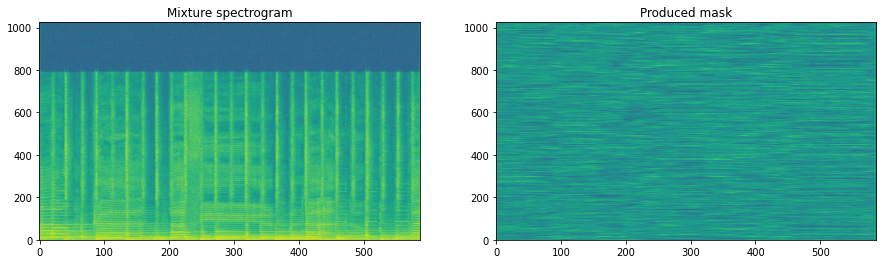
As our model is currently untrained, the produced mask is completely random.

Applying the mask¶

The final step in the model is to actually apply the mask to the mixture representation. Using the steps we talked about before, let’s put that in the model code:

from nussl.ml.networks.modules import Embedding

class Model(nn.Module):
    def __init__(self, num_features, num_audio_channels, hidden_size,
                 num_layers, bidirectional, dropout, num_sources, 
                activation='sigmoid'):
        super().__init__()
        
        self.amplitude_to_db = AmplitudeToDB()
        self.input_normalization = BatchNorm(num_features)
        self.recurrent_stack = RecurrentStack(
            num_features * num_audio_channels, hidden_size, 
            num_layers, bool(bidirectional), dropout
        )
        hidden_size = hidden_size * (int(bidirectional) + 1)
        self.embedding = Embedding(num_features, hidden_size, 
                                   num_sources, activation, 
                                   num_audio_channels)
        
    def forward(self, data):
        mix_magnitude = data # save for masking
        
        data = self.amplitude_to_db(mix_magnitude)
        data = self.input_normalization(data)
        data = self.recurrent_stack(data)
        mask = self.embedding(data)
        
        estimates = mix_magnitude.unsqueeze(-1) * mask
        return estimates

nb, nt, nf, nac = mix_tensor.shape
model = Model(nf, nac, 50, 2, True, 0.3, 1, 'sigmoid')
output = model(mix_tensor)

print_stats(mix_tensor)
print_stats(output)

Shape: torch.Size([1, 587, 1025, 2])
Mean: 0.00044009656994603574
Var: 6.760465112165548e-06

Shape: torch.Size([1, 587, 1025, 2, 1])
Mean: 0.00022057410387787968
Var: 1.7174875210912433e-06

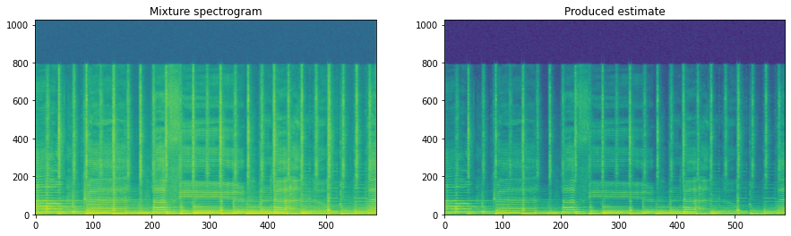
Let’s take a look at the produced estimate:

estimate = to_numpy(output[0, ..., 0])

fig, ax = plt.subplots(1, 2, figsize=(15, 4))
ax[0].imshow(20 * np.log10(representation[..., 0]), origin='lower', aspect='auto')
ax[0].set_title('Mixture spectrogram')
ax[1].imshow(20 * np.log10(estimate[..., 0].T), origin='lower', aspect='auto')
ax[1].set_title('Produced estimate')
plt.show()

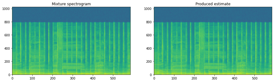
Note

One reason we use masking inside the network is to make life easier for the network. All it has to do for every time-frequency point is to decide whether it belongs or doesn’t belong, rather than trying to estimate the magnitude directly, which can be a much tougher problem to try and solve.

Deep Clustering¶

Deep clustering is an alternative way to train source separation networks. The idea is to project every time-frequency point to a D-dimensional unit-normalized embedding, and then use K-means clustering to extract the actual sources.

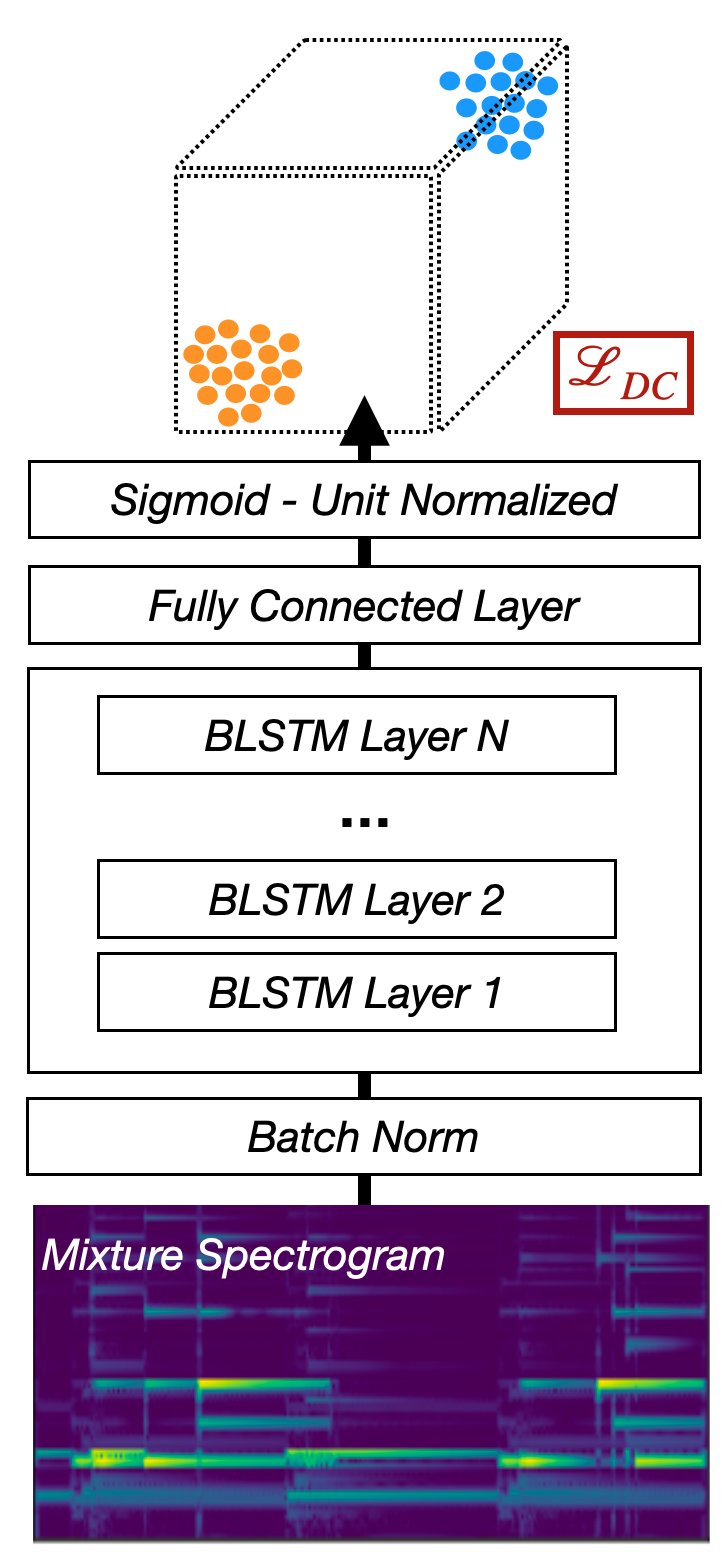
Fig. 50 A diagram of the Deep Clustering architecture.¶

To make our model a deep clustering model, all we have to do is change how the “Embedding” layer works:

from nussl.ml.networks.modules import Embedding

class Model(nn.Module):
    def __init__(self, num_features, num_audio_channels, hidden_size,
                 num_layers, bidirectional, dropout, embedding_size, 
                activation=['sigmoid', 'unit_norm']):
        super().__init__()
        
        self.amplitude_to_db = AmplitudeToDB()
        self.input_normalization = BatchNorm(num_features)
        self.recurrent_stack = RecurrentStack(
            num_features * num_audio_channels, hidden_size, 
            num_layers, bool(bidirectional), dropout
        )
        hidden_size = hidden_size * (int(bidirectional) + 1)
        self.embedding = Embedding(num_features, hidden_size, 
                                   embedding_size, activation, 
                                   num_audio_channels)
        
    def forward(self, data):
        mix_magnitude = data # save for masking
        
        data = self.amplitude_to_db(mix_magnitude)
        data = self.input_normalization(data)
        data = self.recurrent_stack(data)
        mask = self.embedding(data)
        
        estimates = mix_magnitude.unsqueeze(-1) * mask
        return estimates

nb, nt, nf, nac = mix_tensor.shape
model = Model(nf, nac, 50, 2, True, 0.3, 20, ['sigmoid', 'unit_norm'])
output = model(mix_tensor)

print_stats(mix_tensor)
print_stats(output)

Shape: torch.Size([1, 587, 1025, 2])
Mean: 0.00044009656994603574
Var: 6.760465112165548e-06

Shape: torch.Size([1, 587, 1025, 2, 20])
Mean: 9.840189886745065e-05
Var: 3.380243072115263e-07

The output of the network are now 20-dimensional time-frequency points. We can visualize the embedding space using PCA (Principle Component Analysis):

from sklearn.decomposition import PCA

np_output = to_numpy(output.reshape(-1, 20))
pca = PCA(n_components=2)
pca_output = pca.fit_transform(np_output)

plt.scatter(pca_output[:, 0], pca_output[:, 1])
plt.xlabel('PCA Component 1')
plt.ylabel('PCA Component 2')
plt.title('PCA of embedding space')
plt.show()

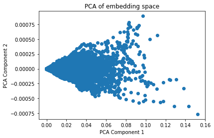
Since we haven’t trained the network at all, yet, it’s just a big blob (one cluster). With a trained network, you’d see multiple tight clusters.

Deep audio estimation¶

In recent years, the trend has gone towards learning to output the waveform directly. In this part, we’ll build up a waveform in/waveform out model by adding components to our already built mask estimation model.

Taking the STFT/iSTFT in a forward pass¶

The first step in creating a waveform in/waveform out model is to move the computation of the STFT and inverse STFT inside the model function. nussl has an STFT module built in with both directions (transform and inverse) implemented. nussl’s implementation is built to match the Scipy STFT implementation as close as possible. Let’s use it:

from nussl.ml.networks.modules import STFT

stft = STFT(2048, hop_length=512)
mix_audio = torch.from_numpy(item['mix'].audio_data).unsqueeze(0).float()
scipy_mag = np.abs(item['mix'].stft())
torch_stft = stft(mix_audio, direction='transform')
print(torch_stft.shape, scipy_mag.shape)

torch.Size([1, 587, 2050, 2]) (1025, 587, 2)

There are a few things to note here:

The ordering of dimensions is different. In the torch STFT, the time axis goes second and the frequency axis third. There’s also a batch dimension.
The torch STFT has twice the features along the frequency dimension. This is because the first half are the magnitude features and the second half are the phase features.

Let’s compute the magnitude spectrogram of the torch STFT:

nb, nt, nf, nac = torch_stft.shape
# Stack the real/imag along the second to last axis
torch_stft = torch_stft.reshape(nb, nt, 2, -1, nac)
print(torch_stft.shape)
# Compute the magnitude
torch_mag, torch_phase = torch_stft[:, :, 0, ...], torch_stft[:, :, 1, ...]
print(torch_mag.shape)

fig, ax = plt.subplots(1, 2, figsize=(15, 4))
ax[0].imshow(20 * np.log10(scipy_mag[..., 0]), origin='lower', aspect='auto')
ax[0].set_title('Mixture spectrogram')
ax[1].imshow(20 * np.log10(torch_mag[0, ..., 0].T), origin='lower', aspect='auto')
ax[1].set_title('Produced estimate')
plt.show()

torch.Size([1, 587, 2, 1025, 2])
torch.Size([1, 587, 1025, 2])

np.abs(torch_mag[0, ...,].permute(1, 0, 2).numpy() - scipy_mag).max()

3.4782241475905806e-08

Above, you can see the error between torch STFT and scipy STFT is on the order of 1e-8. Now, let’s modify our model so that it takes the STFT and iSTFT:

from nussl.ml.networks.modules import Embedding

class Model(nn.Module):
    def __init__(self, num_features, num_audio_channels, hidden_size,
                 num_layers, bidirectional, dropout, embedding_size, 
                 num_filters, hop_length, window_type='sqrt_hann', # New STFT parameters
                 activation=['sigmoid', 'unit_norm']):
        super().__init__()
        
        self.stft = STFT(
            num_filters, 
            hop_length=hop_length, 
            window_type=window_type
        )
        self.amplitude_to_db = AmplitudeToDB()
        self.input_normalization = BatchNorm(num_features)
        self.recurrent_stack = RecurrentStack(
            num_features * num_audio_channels, hidden_size, 
            num_layers, bool(bidirectional), dropout
        )
        hidden_size = hidden_size * (int(bidirectional) + 1)
        self.embedding = Embedding(num_features, hidden_size, 
                                   embedding_size, activation, 
                                   num_audio_channels)
        
    def forward(self, data):
        # Take STFT inside model
        mix_stft = self.stft(data, direction='transform')
        nb, nt, nf, nac = mix_stft.shape
        # Stack the mag/phase along the second to last axis
        mix_stft = mix_stft.reshape(nb, nt, 2, -1, nac)
        mix_magnitude = mix_stft[:, :, 0, ...] # save for masking
        mix_phase = mix_stft[:, :, 1, ...] # save for reconstruction
        
        data = self.amplitude_to_db(mix_magnitude)
        data = self.input_normalization(data)
        data = self.recurrent_stack(data)
        mask = self.embedding(data)
        
        # Mask the mixture spectrogram
        estimates = mix_magnitude.unsqueeze(-1) * mask
        
        # Recombine estimates with mixture phase
        mix_phase = mix_phase.unsqueeze(-1).expand_as(estimates)
        estimates = torch.cat([estimates, mix_phase], dim=2)
        estimate_audio = self.stft(estimates, direction='inverse')
        
        return estimate_audio

model = Model(1025, 2, 50, 2, True, 0.3, 2, 2048, 512)
output = model(mix_audio)

print_stats(mix_tensor)
print_stats(output)

Shape: torch.Size([1, 587, 1025, 2])
Mean: 0.00044009656994603574
Var: 6.760465112165548e-06

Shape: torch.Size([1, 2, 300032, 2])
Mean: 1.817797965486534e-05
Var: 0.005776260048151016

There’s a bit of tricky business in recombining the magnitude and phase features for reconstructing the estimates. However, this network is functionally identical to the previous one - all that’s changed is that we’re taking the STFT and iSTFT within the network! Let’s listen to the output:

for i in range(output.shape[-1]):
    source = output[0, ..., i]
    nussl.AudioSignal(audio_data_array=to_numpy(source), sample_rate=44100).embed_audio()

As these networks are not trained, the output is basically still the mixture.

Learned filterbanks¶

The next major step forward in the source separation literature was learnable filterbanks. Rather than take just an STFT, people discovered that learning the representation jointly with the output audio provided even better separation results - sometimes better than an oracle time-frequency mask!

To understand how this works, lets delve into the math of the STFT a tiny bit. The most common way of calculating the STFT is to take the following steps:

Window the signal into small overlapping windows
Compute the FFT of each window individually
Each FFT becomes a frame of the STFT

The operation here looks a bit like a convolution, actually!

Break up signal into small overlapping windows (stride of convolution == hop length of the STFT).
Cross-correlate each window with a set of learned filters.
The response of all the filters for each window becomes a “frame”.

The connection between the STFT and the learned filterbank is inside step 2: what filters of a convolution correspond to doing a Fourier transform?

A Fourier transform breaks up a signal into the sum of sinusoids at different weights and offsets. By making our convolutional filters equal to a bunch of sinusoids, we can replicate the STFT as a matrix multiplication:

filter_length = 128

fig, ax = plt.subplots(8, 8, figsize=(12, 10))
ax = ax.flatten()

fourier_basis = torch.fft.rfft(
    torch.eye(filter_length)
)
cutoff = 1 + filter_length // 2
fourier_basis = torch.cat([
    torch.real(fourier_basis[:, :cutoff]),
    torch.imag(fourier_basis[:, :cutoff])
], dim=1)
fourier_basis = fourier_basis.float()

for i in range(ax.shape[-1]):
    ax[i].plot(to_numpy(fourier_basis)[:, i])
    ax[i].set_xticks([])
    ax[i].set_yticks([])
plt.suptitle('Convolutional filters for a Fourier transform', fontsize=16)
plt.tight_layout()
plt.show()

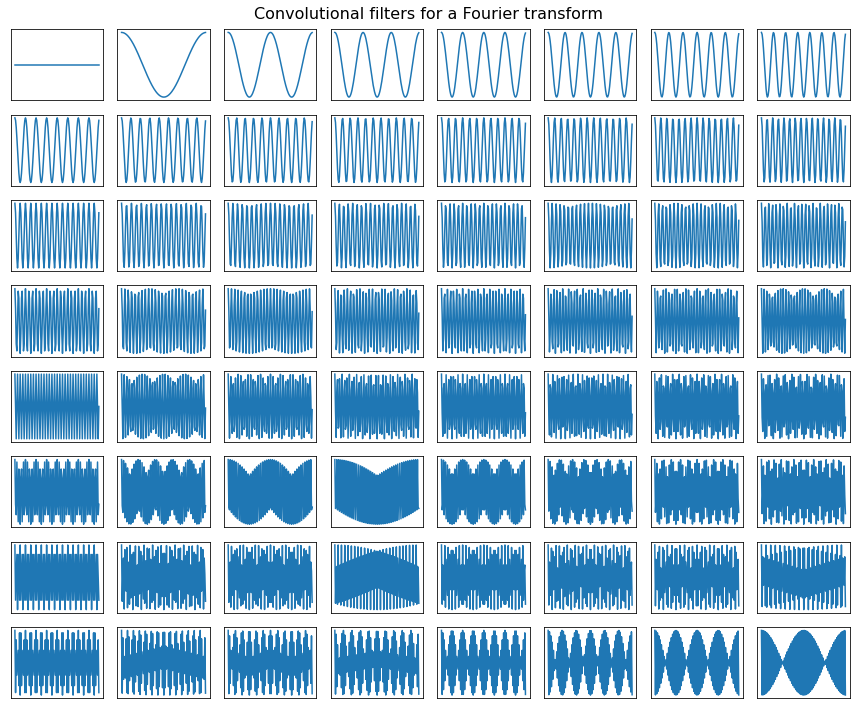
The next step is make these filters learnable, by initializing them randomly. We can do this by replacing the nussl STFT module with its LearnedFilterBank module:

from nussl.ml.networks.modules import LearnedFilterBank

class Model(nn.Module):
    def __init__(self, num_features, num_audio_channels, hidden_size,
                 num_layers, bidirectional, dropout, embedding_size, 
                 num_filters, hop_length, window_type='rectangular', # Learned filterbank parameters
                 activation=['sigmoid', 'unit_norm']):
        super().__init__()
        
        self.representation = LearnedFilterBank(
            num_filters, 
            hop_length=hop_length, 
            window_type=window_type
        )
        self.amplitude_to_db = AmplitudeToDB()
        self.input_normalization = BatchNorm(num_features)
        self.recurrent_stack = RecurrentStack(
            num_features * num_audio_channels, hidden_size, 
            num_layers, bool(bidirectional), dropout
        )
        hidden_size = hidden_size * (int(bidirectional) + 1)
        self.embedding = Embedding(num_features, hidden_size, 
                                   embedding_size, activation, 
                                   num_audio_channels)
        
    def forward(self, data):
        # Take STFT inside model
        mix_repr = self.representation(data, direction='transform')
        
        data = self.amplitude_to_db(mix_repr)
        data = self.input_normalization(data)
        data = self.recurrent_stack(data)
        mask = self.embedding(data)
        
        # Mask the mixture spectrogram
        estimates = mix_repr.unsqueeze(-1) * mask
        
        # Recombine estimates with mixture phase
        estimate_audio = self.representation(estimates, direction='inverse')
        
        return estimate_audio

model = Model(128, 2, 50, 2, True, 0.3, 2, 128, 32)
output = model(mix_audio)

print_stats(mix_tensor)
print_stats(output)

Shape: torch.Size([1, 587, 1025, 2])
Mean: 0.00044009656994603574
Var: 6.760465112165548e-06

Shape: torch.Size([1, 2, 300032, 2])
Mean: 0.001926163793541491
Var: 25.08449935913086

Note that LearnedFilterBanks don’t have a strict concept of “phase” vs “magnitude”. Instead, they learn the two aspects jointly.

Open-Source Tools & Data for Music Source Separation

Coding up model architectures¶

Deep mask estimation¶

Model overview¶

Masking¶

Log-magnitude representation¶

Input normalization¶

Recurrent processing¶

Mapping to a mask¶

Applying the mask¶

Deep Clustering¶

Deep audio estimation¶

Taking the STFT/iSTFT in a forward pass¶

Learned filterbanks¶