Architectures
We now have the conceptual building blocks in place to understand many of the modern deep learning systems for source separation. In this section, we will outline a few of the recent systems.
These architectures, like all source separation approaches, are divided into systems that make masks that are applied to the mixture spectrogram, and those that estimate the source waveforms directly. All of the same concepts that we’ve explored in the Classic approaches section still apply; now we’re just using a more powerful system (i.e., neural nets) to make a high dimensional representations that we can separate.
Mask-Based Systems
U-Net & Friends
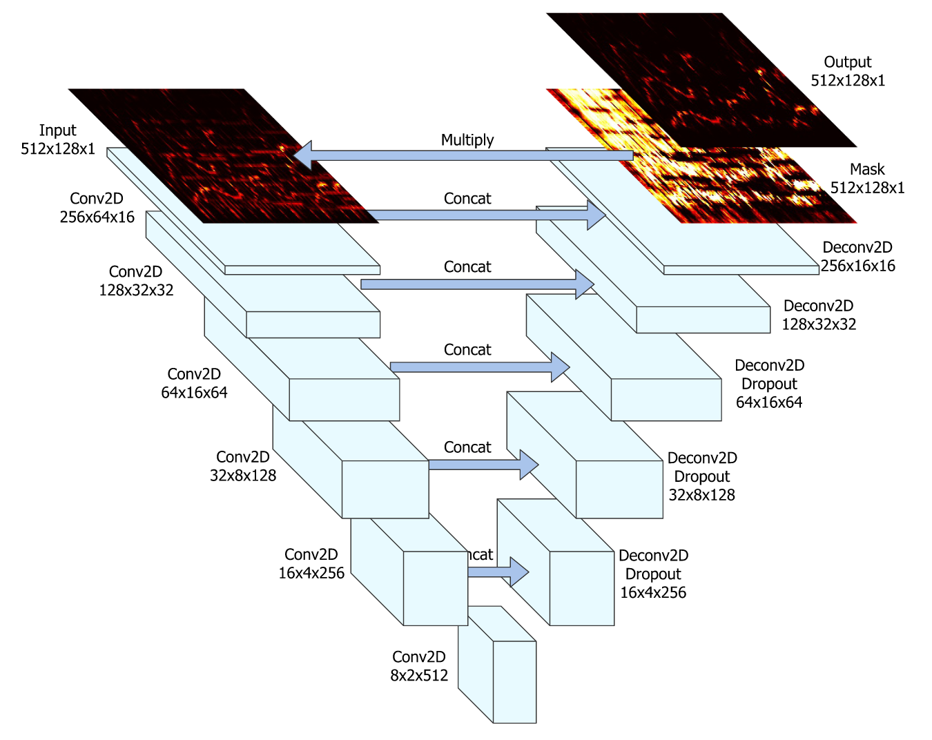
Fig. 36 The U-Net architecture. Image used courtesy of Rachel Bittner.
U-Nets [JHM+17] are a very popular architecture for music source separation systems. The popular source separation system Spleeter by Deezer uses this network architecture. [HKVM20]
U-Nets input a spectrogram and perform a series of 2D convolutions, each of which producing an encoding of a smaller and smaller representation of the input. The small representation at the center is then scaled back up by decoding with the same number of 2D deconvolutional layers (sometimes called transpose convolution), each of which corresponds to the shape of one of the convolutional encoding layers. Each of the encoding layers is concatenated to the corresponding decoding layers.
The original U-Net paper [JHM+17] has 6 strided 2D convolutional encoder layers with 5x5 kernel sizes and strides of 2. After each encoder layer was a batch norm followed by a ReLU activation. A Dropout of 50% is applied to the first three encoder layers. After the 6th encoder layer, 5 decoder layers with the same kernel and stride sizes, also with batch norm and ReLU activations. The final layer has a sigmoid activation function that makes a mask.
The final mask is multiplied by the input mixture and the loss is taken between the ground truth source spectrogram and mixture spectrogram with the estimated mask applied, as per usual.
Because the U-Net is convolutional, it must process a spectrogram that has a fixed shape. In other words, an audio signal must be broken up into spectrograms with the same number of time and frequency dimensions that the U-Net was trained with.
Variants
Many variants of the U-Net architecture have been proposed. A few recent papers have added a method of controlling the output source by conditioning the network. [SHGomez20,PCC+20,MBP19] Conditioning means providing additional information to the network; we add a control module to the network that allows us to tell it which source we want it to separate.
Other variants include U-Nets that separate multiple sources at once (as opposed to one network per source) [KMHGomez20], jointly learning the fundamental frequency of the singing voice [JBEW19], jointly learning instrument [HL20] or singing voice activity [SED18a].
Some of these variants follow the neural network details outlined above (which are taked from the original U-Net paper [JHM+17]), but some use different activation functions or do multiple convolutional layers before concatenating to the respective deconvolutional layer.
Open-Unmix
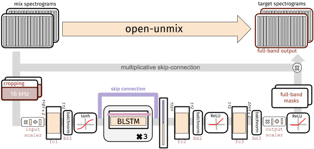
Fig. 37 A diagram showing the Open-Unmix architecture for source separation. Image used courtesy of Fabian-Robert Stöter (source).
Open-Unmix is a more recent neural network architecture that boasts impressive
performance. Open-Unmix has one fully connected layer with batch norm and a tanh
activation, followed a set of three BLSTM layers in the center, and then two
more fully connected layers with batch norm and ReLU activations. The pytorch
implementation has a dropout applied to the first two BLSTM layers with a
zeroing probability of 40%.
There are a few things of note about the Open-Unmix architecture: first, are the fully connected layers before the BLSTM layers. The output of these layers is smaller than the input frequency dimension (the time dimension is unchanged). This compresses the representation that the BLSTM layers are learning from, which should be a more distilled representation of the the audio.
Second, is the skip connection around the BLSTM layers, which allows the network to learn whether or not using those layers are helpful (it “skips” the BLSTMs).
Finally, note that there a normalization functions throughout the architecture. Recall that normalization helps neural networks learn because then the inputs are always within a well defined region. Global normalization steps occur before the first fully connected layer and right at the end, and in between there are batch normalization layers.
Mask Inference
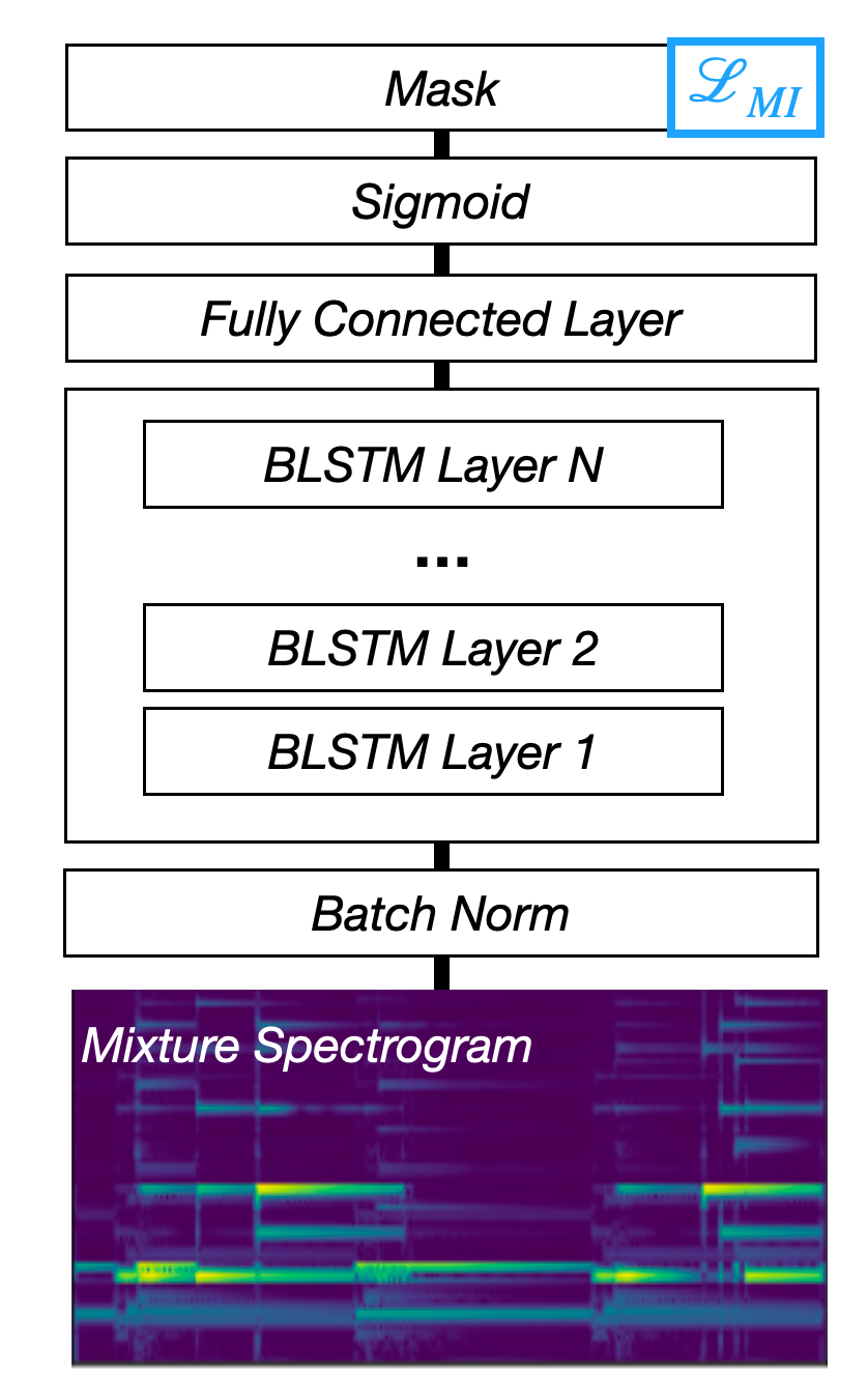
Fig. 38 A diagram of the Mask Inference architecture.
Although many deep learning systems make masks, the term Mask Inference typically refers to a specific type of source separation architecture. Mask Inference networks input a spectrogram, which is fed into a handful of recurrent neural network layers that are connected to a fully connected layer that outputs the mask. It is common to use Bidirectional Long Short-term Memory (BLSTM) networks as the recurrent layers. As mentioned, this gives the network twice as many trainable parameters; one set going forward in time and another going backward in time. The fully connected layer then converts the output of the BLSTM to the shape of the spectrogram to make a mask. It is typical to use sigmoid activation on the fully connected layer to create the mask.
A standard architecture for a Mask Inference is shown in the figure above. It inputs a magnitude spectrogram, applies batch normalization, goes to 4 BLSTM layers, then to a fully connected layer with a sigmoid activation function. A dropout of 30% zeroing probability is applied to the first 3 BLSTM layers.
Mask Inference networks are usually trained with an \(L_1\) loss between the estimated spectrogram (i.e., the estimated mask element-wise multiplied by the mixture spectrogram) and the target spectrogram. Although it is a bit of a misnomer, this loss is called a Mask Inference Loss.
Deep Clustering
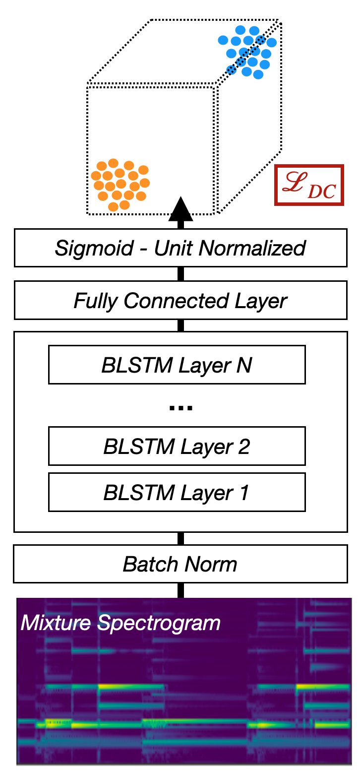
Fig. 39 A diagram of the Deep Clustering architecture.
Deep Clustering maps each TF bin to a high-dimensional embedding space such that TF bins dominated by the same source are close and those dominated by different sources are far apart. We say that a TF bin is dominated by some Source \(S_i\) if most of the energy in that source is from \(S_i\).
Deep Clustering has the same basic network architecture as a Mask Inference network: spectrogram input, to batch norm, to a set of BLSTM layers to a fully connected layer. The catch here is that deep clustering needs to project each TF bin to a high dimensional space. So for a 20 dimensional embedding space, the output size of the fully connected layer is \(T \times F \times 20\). The deep clustering loss is applied to this high dimensional output of the embedding space.
Once the network is trained to make the embedding space, a separate clustering algorithm like k-means must be applied to the embedding space to make masks.
Chimera
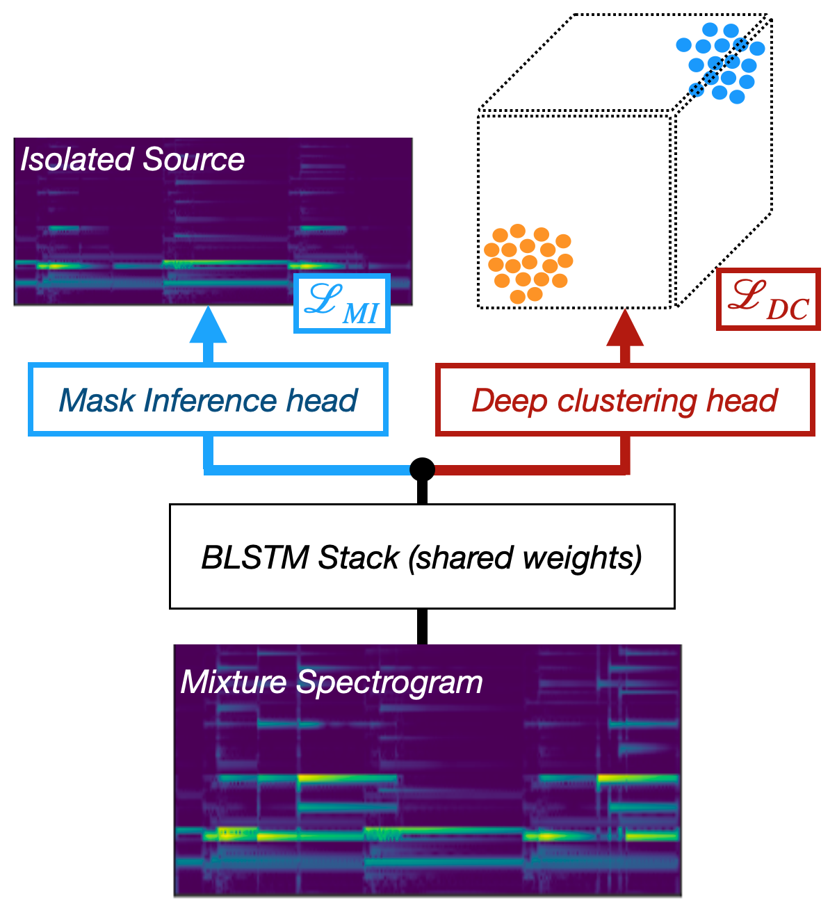
Fig. 40 A diagram of the Chimera architecture.
Chimera [LCH+17] combines the Mask Inference and Deep Clustering architectures into a multi-task neural network. The net is trained to optimize both loss functions simultaneously. It does this by having a separate “head” for each loss. Each of these heads is its own fully connected layer and activation with a shared set of BLSTM weights, usually set up the same way as Mask Inference or Chimera above. In this instance we don’t use the deep clustering head to produce masks, but rather we only use the Mask Inference head. During training the Deep Clustering head acts as a regularizer that helps the network generalize to unseen mixes.
Waveform Systems
Tasnet & Friends
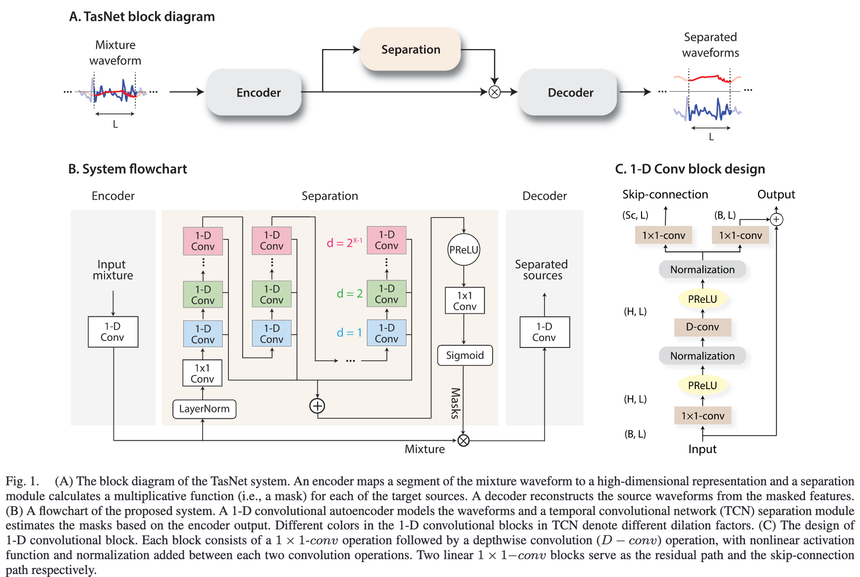
Fig. 41 A diagram showing the ConvTasnet architecture. Image used courtesy of Yi Luo.
The Tasnet [LM18] is a speech separation architecture that is structured very similar the Mask Inference architecture outlined above, with LSTM layers at the center. Tasnet has one main difference: Tasnet used a pair of convolutional layers to input and output waveforms directly. Additionally, because Tasnet outputs the waveforms directly it doesn’t need the additional step of multiplying by a mixture STFT to get the phase information.
ConvTasnet [LM19] is the second iteration of the original TasNet speech separation architecture. It replaces the LSTM center of Tasnet with 1D convolutional layers that separate the input signal.
While both Tasnet and ConvTasnet have both been popular in the speech separation literature, to our knowledge only ConvTasnet has seen use in music separation based on its implementation by the authors of Demucs [DefossezUBB19b]. This is because the translation from speech to music was not so straight forward in this case.
ConvTasnet and Tasnet both use SI-SNR loss between target and estimated waveforms.
Wave-U-Net
Wave-U-Net [SED18b] is an extension of the U-Net architecture that operates directly on waveforms. Instead of 2D convolutions/deconvolutions acting on a spectrogram, Wave-U-Nets have a series of 1D convolutions/deconvolutions that operate on audio directly. Just like the spectrogram U-Net though, the convolutional encoding layers are concatenated with the corresponding deconvolutional decoding layers.
Wave-U-Net uses MSE loss between the target and estimated waveforms.
Demucs
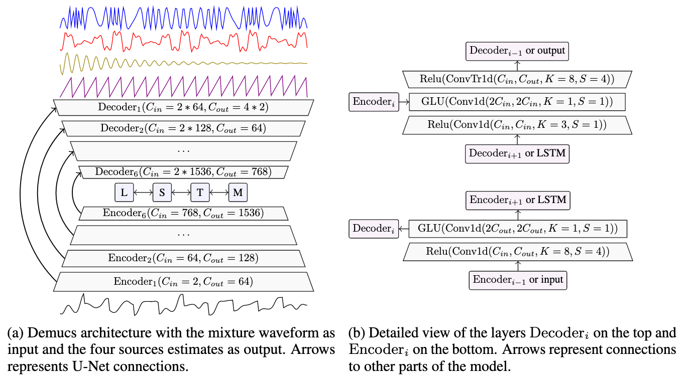
Fig. 42 A diagram showing the original Tasnet architecture. Image used courtesy of Alexandre Défossez.
Demucs [DefossezUBB19a,DefossezUBB19b] is similar to both Wave-U-Net and Tasnet. It has the skip connections just as in Wave-U-Net, but at the center it has two BLSTM layers. The specific details of the shape of each layer are shown in the diagram.
The Demucs authors recently released a real-time version of this architecture for speech enhancement. Training a similar model for music could be an exciting development that enables more applications in source separation.
Demucs uses \(L_1\) loss between the target and estimated waveform, scaled by the length (in samples) of the signals.
Next Steps…
This wraps up this section of the tutorial. Over the next few sections we will get some hands-on experience building these kinds of models. Before we get to writing model code, though, there’s one very important factor about these systems that we haven’t covered yet: data!
Coming up, we’ll cover how to use Scaper to create large, augmented data sets, and after that we’ll wrap up with how to put together and train a model like the ones on this page.