Phase
While many source separation papers mainly focus on their approaches for creating better mask estimates, which only apply to the magnitude components of a TF Representation, the other crucial aspect of sound is its phase.
In this section, we will discuss the important problem of how to turn a magnitude spectrogram of an estimated source back into a waveform so that we may listen to the source estimation.
Phase - A Quick Primer
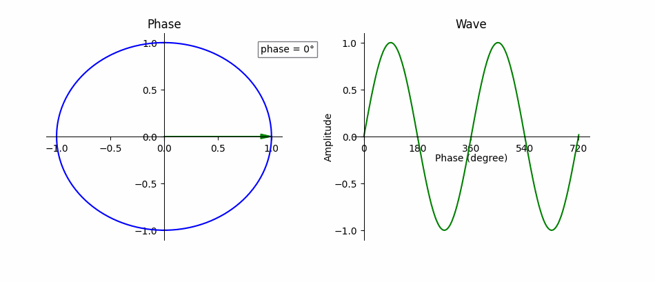
Fig. 16 Phase is the instantaneous amplitude of an audio signal. Phase is a fundamental part of representing the signal. Adapted from Wikimedia.
An audio signal, \(y(t)\), composed of exactly one sine wave,
can be completely described by the parameters \(t, A, f\) and \(\phi\), where \(t\) represents time in seconds, \(A\) is the wave’s amplitude (unit-less), \(f\) is its frequency in Hz, and \(\phi\) is its phase offset in radians (i.e., where in the cycle the wave is at \(t=0\)). If \(\phi \ne 0\), then the sine wave appears shifted in time by \(\frac{\phi}{2 \pi f}\), where negative values “delay” the signal and positive values “advance” it. Recall that a sine wave is the same value every \(2 \pi f\) seconds, i.e.
This is inherent the periodicity of the sine wave, and the point where the phase “wraps around” or essentially restarts at 0 every \(2 \pi f\) seconds.
Let’s scale this up. Our old pal Fourier told us that any sound can be represented as an infinite summation of sine waves each with their own amplitudes, frequencies, and phase offsets. This means that any sound we hear can be represented as many, many tuples of \((t, A, f, \phi)\).
Let’s think back to the section about time-frequency representations: each bin is index by time along the x-axis and frequency along the y-axis. We’ll be a little hand-wavy here, but we can think of a TF bin as a “snapshot” of the sound at that particular time and at that particular frequency component. In a magnitude spectrogram, power spectrogram, log spectrogram, etc, each value represents the sound’s energy for that frequency at that time. So, if you’re keeping track at home, a spectrogram has entries for \(t, A\) and \(f\), but no representation for the phase \(\phi\).
Phase is crucial to be able to describe and audio signal. Why don’t most source separation approaches model phase information?
Why We Don’t Model Phase
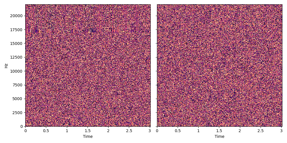
Fig. 17 The structure of phase within an STFT makes it hard to model. One of these two images shows the phase component of an STFT and another shows random noise. Can you guess which is which?
Let’s do a little experiment. Above are two images. One of the two images shows the phase component of an audio signal, the other shows white noise. Can you guess which is which? 1
Therein lies the problem: there is a complicated interplay between how the DFT captures the signal at each time step, how the frequency is captured and how the phase is captured. Let’s build some intuition for why this is. For the same time step, the lower frequency components of the signal change less quickly than the higher frequency components. This means that for any two adjacent time steps, the time difference is the same but the amount of change of any frequency might not be the same. The phase wraparound happens much quicker at the higher frequencies than at the lower frequencies.
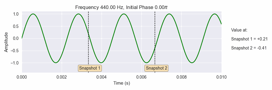
Fig. 18 Getting a snapshot of the phase (the black dotted vertical lines) is very sensitive to the frequencies and initial phases of the sine waves. This is similar to what happens when take an STFT: many snapshots of sine waves with many frequencies and initial phase offsets.
The gif above shows a sine wave with varying frequency and initial phase. The frequency starts at A440, or 440 Hz and gradually changes frequency up an octave higher (880 Hz). The initial phase also changes in the interval \([0.0, 2\pi]\). The dotted black lines show two shapshots of the value of the sine wave as the frequency and initial phase both change. Notice how sensitive the snapshot are to changes in the frequency and initial phase.
Another big difficulty when dealing with phase is that humans do not always perceive phase differences, i.e., a sine wave with \(\phi = 0\) sounds the same as a sine wave with \(\phi' \ne 0\)
This is all to say that getting phase right is hard. That being said, there are ways to estimate phase, but few if any source separation approaches (or sound generation models) attempt to explicitly model phase to the same extent that magnitude information is modeled. We will discuss some of these phase estimation techniques below.
How to Deal with Phase
The Easy Way
For a mask-based source separation approach, a easy and very common way to deal with phase is to just copy the phase from the mixture! The mixture phase is sometimes referred to as the noisy phase. This strategy isn’t perfect, but researchers have discovered that it works surprisingly well, and when things go wrong, it’s usually not the fault of the phase.
So now, with this in place, we finally have our first strategy to convert our source estimate back to a waveform. Assume we have a mixture STFT, \(Y \in \mathbb{C}^{T \times F}\), and estimated mask \(\hat{M}_i \in [0.0, 1.0]^{T \times F}\) for Source \(i\). Recall that we can apply the mask to a magnitude spectrogram of \(Y\) like so:
where \(\hat{X}_i \in \mathbb{R}^{T \times F}\) represents a magnitude spectrogram of our source estimate. Note that this equation looks similar if we want to apply a mask to a power spectrogram (\(|Y|^2\)), log spectrogram (\(\log |Y|\)), etc.
Now we can just copy the phase from the mixture over to the magnitude spectrogram of our source estimate, \(\hat{X}_i\):
where we use \(j = \sqrt{-1}\), “\(\angle\)” to represent the angle of the complex-valued STFT of \(Y\), and \(\tilde{X}_i \in \mathbb{C}^{T \times F}\) to indicate that the estimate for Source \(i\) is now complex-valued similar to an STFT.
Putting it all together it looks like:
This math looks pretty complicated, but this is really just a few lines of code:
def apply_mask_with_noisy_phase(mix_stft, mask):
    mix_magnitude, mix_phase = np.abs(mix_stft), np.angle(mix_stft)
    src_magnitude = mix_magnitude * mask
    src_stft = src_magnitude * np.exp(1j * mix_phase)
    return src_stft
The Hard Way, Part 1: Phase Estimation
It is possible to estimate the phase once the estimated mask is applied to the mixture spectrogram. One popular way is the Griffin-Lim algorithm [GL84], which attempts to reconstruct the phase component of a spectrogram by iteratively computing an STFT and an inverse STFT. Griffin-Lim usually converges in 50-100 iterations, although faster methods have been developed [PBSondergaard13]. In our experience, Griffin-Lim can still leave artifacts in the audio.
Tip
librosa has an implementation of Griffin-Lim here.
Multiple Input Spectrogram Inversion (MISI) is a variant of Girffin-Lim specifically designed for source separation with multiple sources. It adds an additional constraint to the original algorithm such that all of the estimated sources with estimated phase components must all add up to the input mixture. [GS10]
It’s worth noting that the STFT & iSTFT computations, and these phase estimation algorithms are all differentiable. This means that we can incorporate them as part of neural network architectures and train directly on the waveforms, even when using mask-based algorithms. [WLR18,LRWW+19,MYK+19]
The Hard Way, Part 2: Waveform Estimation
Finally, a recent way that researchers have been tackling the phase problem is by side-stepping any explicit representations of it at all. Recently, many deep learning-based models have been proposed that are “end-to-end”, meaning that the model’s input and output are all waveforms. In this case, the model decides how it wants to represent phase. This might not always be the most efficient or effective solution, although many ways to mitigate the drawbacks of this tactic are currently being researched. [EAC+18,EGR+19]
- 1
We won’t keep you guessing forever: the real phase is on the left. This signal was converted from an mp3 so there is a low-pass shelf at ~17 kHz, which is noticeable once you know what you’re looking for. There is no data above the shelf though, so this is actually an artifact, not a true representation of the signal.