Putting it All Together: Repetition¶

So far, we have learned about the concepts behind source separation, but now let’s put everything together and get a feel for how the ideas all work in practice. In this section, we will synthesize all the ideas of the previous sections; we will examine and compare three similar algorithms on the same song. We hope to provide you with some intuition about how all the pieces fit together.

Repetition¶

Repetition is a common feature of almost every type of music. Oftentimes, we can use this cue to identify different sources in a song: a trumpet might improvise a new melody over a backing band that is repeating the same few bars. In this case, we can leverage the repetition of the backing band to isolate the trumpet.

With that in mind, we will explore three algorithms that attempt to separate a repeating background from a non-repeating foreground. The basic assumptions here are:

that there is repetition in the mixture, and
the repetition captures what we want to separate.

These assumptions hold quite well if we want to separate a trumpet from a backing band, but might not work if we want to isolate a drum set from the rest of the band because the drum set is usually playing a repeating pattern.

Setup¶

The three algorithms we will look at in this section all input magnitude spectrograms from a mixture, try to find the repeating parts in the mixture, and separate them out by creating a mask for the foreground and background. Here we’ll attempt to try to separate a singer from the background instruments.

REPET Overview¶

The first algorithm we will explore here is called the REpeating Pattern Extraction Technique or REPET [RP12b]. REPET works like this:

Find a repeating period, \(t_r\) seconds (e.g., the number of seconds which a chord progression might start over).
Segment the spectrogram into \(N\) segments, each with \(t_r\) seconds in length.
“Overlay” those \(N\) segments.
Take the median of those \(N\) stacked segments and make a mask of the median values.

We’ll use REPET to demonstrate how to run a source separation algorithm in nussl.

%%capture
!pip install git+https://github.com/source-separation/tutorial

# Do our imports
import warnings
warnings.simplefilter('ignore')
import nussl
import matplotlib.pyplot as plt
import numpy as np
from pprint import pprint
from common import viz

Our Input Mixture¶

Let’s download an audio file that has a lot of repetition in it, and inspect and listen to it:

# This example is from MUSDB18. We will discuss this in a later section.
musdb = nussl.datasets.MUSDB18(download=True)
item = musdb[40]

# Get the mix and sources
mix = item['mix']
sources = item['sources']

# Listen to the audio
mix.embed_audio()

# Visualize the spectrogram
plt.figure(figsize=(10, 3))
plt.title('Mixture spectrogram')
nussl.utils.visualize_spectrogram(mix, y_axis='mel')
plt.tight_layout()
plt.show()

Using REPET in `nussl`¶

Now we need to instantiate a Repet object in nussl. We can do that like so:

repet = nussl.separation.primitive.Repet(mix)

Now the repet object has our AudioSignal, it’s easy to run the algorithm:

# Background and Foreground Masks
bg_mask, fg_mask = repet.run()
print(type(bg_mask))

<class 'nussl.core.masks.soft_mask.SoftMask'>

Oh, look! The repet object returned masks! Woohoo!

Applying the Masks¶

Now that we have masks, we can apply them to the mix to get source estimates.

Without Phase¶

Let’s apply the masks to the mixture spectrogram without considering the phase.

# Get the mask numpy arrays
bg_mask_arr = bg_mask.mask
fg_mask_arr = fg_mask.mask

# Multiply the masks to the magnitude spectrogram
mix.stft()
mix_mag_spec = mix.magnitude_spectrogram_data
bg_no_phase_spec = mix_mag_spec * bg_mask_arr
fg_no_phase_spec = mix_mag_spec * fg_mask_arr

# Make new AudioSignals for background and foreground without phase
bg_no_phase = mix.make_copy_with_stft_data(bg_no_phase_spec)
_ = bg_no_phase.istft()
fg_no_phase = mix.make_copy_with_stft_data(fg_no_phase_spec)
_ = fg_no_phase.istft()

Let’s hear what these source estimates sound like:

print('REPET Background without Phase')
_ = bg_no_phase.embed_audio()

print('REPET Foreground without Phase')
_ = fg_no_phase.embed_audio()

REPET Background without Phase

REPET Foreground without Phase

Not bad, but… not great! The phase artifacts are much more apparent in the foreground.

With the Mixture Phase¶

Let’s apply the mixture phase to our estimates. We can use the function we talked about earlier:

def apply_mask_with_noisy_phase(mix_stft, mask):
    mix_magnitude, mix_phase = np.abs(mix_stft), np.angle(mix_stft)
    src_magnitude = mix_magnitude * mask
    src_stft = src_magnitude * np.exp(1j * mix_phase)
    return src_stft

bg_stft = apply_mask_with_noisy_phase(mix.stft_data, bg_mask_arr)
fg_stft = apply_mask_with_noisy_phase(mix.stft_data, fg_mask_arr)


# Make new AudioSignals for background and foreground with phase
bg_phase = mix.make_copy_with_stft_data(bg_stft)
_ = bg_phase.istft()
fg_phase = mix.make_copy_with_stft_data(fg_stft)
_ = fg_phase.istft()

Again, let’s hear the results:

print('REPET Background with Phase')
_ = bg_phase.embed_audio()

print('REPET Foreground with Phase')
_ = fg_phase.embed_audio()

REPET Background with Phase

REPET Foreground with Phase

Much better!

The Easy Way¶

nussl provides functionality for all of the issues regarding applying the mask by doing one of the following:

# Will make AudioSignal objects after we're run the algorithm
repet = nussl.separation.primitive.Repet(mix)
repet.run()
repet_bg, repet_fg = repet.make_audio_signals()

# Will run the algorithm and return AudioSignals in one step
repet = nussl.separation.primitive.Repet(mix)
repet_bg, repet_fg = repet()

Evaluation¶

Okay, now let’s evaluate how well our REPET model did. First we will inspect the model’s output:

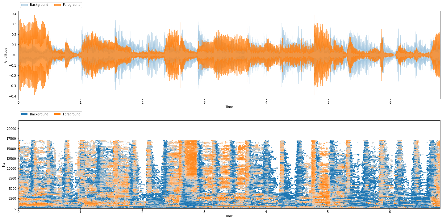
viz.show_sources({'Background': repet_bg, 'Foreground': repet_fg})

Listening to the Ground Truth Sources¶

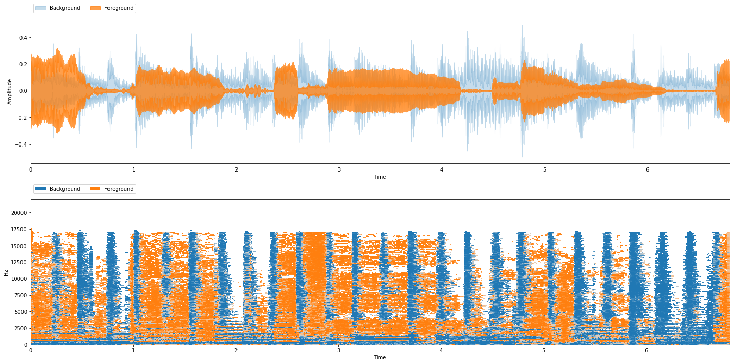
Our example is from MUSDB18 (discussed in detail later) so we have access to this data. Our goal is to separate the singer, so we’ll mix all of the non-vocal sources into the background and call the vocals the foreground:

# Mix the background sources together
gt_bg = sum(src for name, src in sources.items() if name != 'vocals')

gt_bg.path_to_input_file = 'background'  # Label for later

gt_fg = sources['vocals']
gt_fg.path_to_input_file = 'foreground'

Let’s hear what these sound like:

viz.show_sources({'Background': gt_bg, 'Foreground': gt_fg})

SDR & Friends¶

As we mentioned earlier, listening to the output of our model is the best indicator of how well it performs, but SDR & friends can give us an indication of quality as well. Because SDR & friends are so widely used in the literature, let’s take some time and explore how to use it and gain some intuition about its output.

Note

SDR & Friends require access to the ground truth isolated source data.

Let’s evaluate our REPET algorithm using SI-SDR. For historical reasons, all of the SDR-style evaluation functions in nussl are called BSSEval*. We’ll use BSSEvalScale, which has the most recent implementations of SDR, including SI-SDR:

bss_eval = nussl.evaluation.BSSEvalScale(
    true_sources_list=[gt_bg, gt_fg],
    estimated_sources_list=[repet_bg, repet_fg]
)
repet_eval = bss_eval.evaluate()

# Inspect the evaluation
pprint(repet_eval)

{'background': {'MIX-SD-SDR': [3.9314831232234675, 5.336881694926657],
                'MIX-SI-SDR': [3.932129073730801, 5.337614286353903],
                'MIX-SNR': [3.8638559787236137, 5.275643734509963],
                'SD-SDR': [3.5220758723953356, 7.612815648188522],
                'SD-SDRi': [-0.4094072508281319, 2.275933953261865],
                'SI-SAR': [6.279044690434821, 9.308070404907923],
                'SI-SDR': [5.750111670888234, 8.824659887630785],
                'SI-SDRi': [1.8179825971574335, 3.4870456012768827],
                'SI-SIR': [15.155730687012303, 18.598805536773767],
                'SNR': [6.58201457060274, 9.235432372210497],
                'SNRi': [2.7181585918791265, 3.959788637700534],
                'SRR': [7.4871927518943675, 13.748032403948255]},
 'combination': [0, 1],
 'foreground': {'MIX-SD-SDR': [-3.70013700252964, -5.071003563079052],
                'MIX-SI-SDR': [-3.6994910520223083, -5.070270971651808],
                'MIX-SNR': [-3.8638559787236137, -5.275643734509963],
                'SD-SDR': [0.9446974196389686, 2.3142278105338736],
                'SD-SDRi': [4.644834422168609, 7.385231373612926],
                'SI-SAR': [3.7012878072914965, 3.994854150574975],
                'SI-SDR': [1.239971348230485, 2.6645031719579872],
                'SI-SDRi': [4.939462400252793, 7.734774143609795],
                'SI-SIR': [4.878831072535349, 8.45089272807405],
                'SNR': [2.7424917436894116, 3.9932836518827552],
                'SNRi': [6.606347722413025, 9.268927386392718],
                'SRR': [12.767090027543329, 13.421935641611748]},
 'permutation': [0, 1]}

Woah! That’s a lot to look at! We’ll see how to make this look prettier in a later section. For now, let’s just look at SI-SDR, SI-SAR, and SI-SIR:

def print_metrics(eval_dict):
    """Helper function to parse the eval dict"""
    
    # Take mean over channels
    result = f"foreground SI-SDR: {np.mean(eval_dict['foreground']['SI-SDR']):+.2f} dB\n" \
             f"background SI-SDR: {np.mean(eval_dict['background']['SI-SDR']):+.2f} dB\n\n" \
             f"foreground SI-SAR: {np.mean(eval_dict['foreground']['SI-SAR']):+.2f} dB\n" \
             f"background SI-SAR: {np.mean(eval_dict['background']['SI-SAR']):+.2f} dB\n\n" \
             f"foreground SI-SIR: {np.mean(eval_dict['foreground']['SI-SIR']):+.2f} dB\n" \
             f"background SI-SIR: {np.mean(eval_dict['background']['SI-SIR']):+.2f} dB\n"
    print(result)

print_metrics(repet_eval)

foreground SI-SDR: +1.95 dB
background SI-SDR: +7.29 dB

foreground SI-SAR: +3.85 dB
background SI-SAR: +7.79 dB

foreground SI-SIR: +6.66 dB
background SI-SIR: +16.88 dB

Recal that the Signal-to-Distortion Ratio (SDR) is considered “overall quality” of the estimated sources, the Signal-to-Artifacts Ratio (SAR) captures how many unnatural artifacts there are in the sources, and Signal-to-Interference Ratio (SIR) captures how many sounds from other sources are in each source estimate. Higher values are better.

Ask yourself: How do these numbers fit with how you perceived the output quality of our REPET model? Do you feel that the REPET model did a good job separating the singer from everything else in the mixture?

Exercise: Making it Interactive!¶

nussl has hooks for gradio, so we can make our repet object interactive. All algorithms in nussl have this ability.

%%capture
# Comment out the line above to run this cell
# interactively in Colab or Jupyter Notebook

repet.interact(share=True, source='microphone')

Take a few minutes to play around with REPET. See what types of audio work and what types of audio doesn’t work. How does it work on electronic loops? How does it work on ambient music?

REPET-SIM¶

Now let’s look at a few other algorithms that leverage repetition in a musical recording and compare results to REPET.

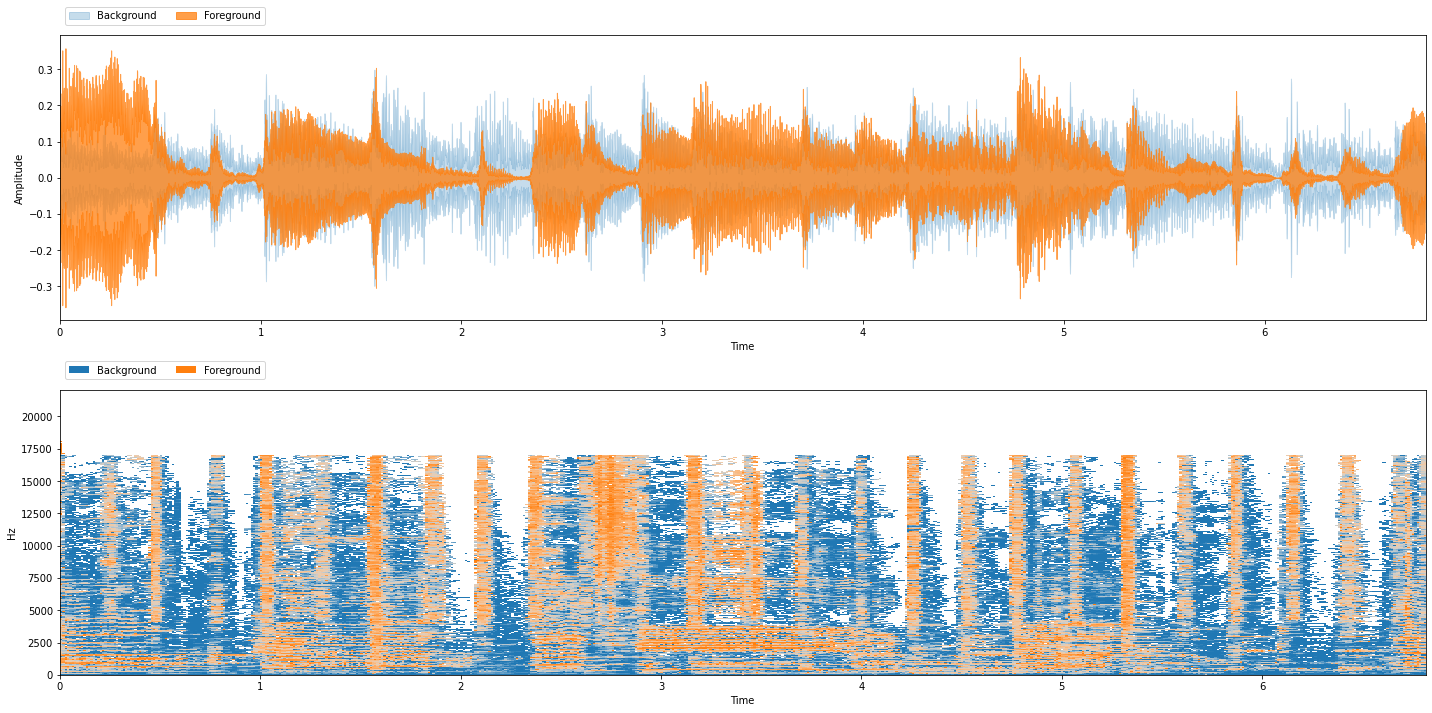
REPET-SIM [RP12a] is a variant of REPET that doesn’t rely on a fixed repeating period. In fact, it doesn’t rely on repetition as explicitly as REPET does. REPET-SIM calculates a similarity matrix between each pair of spectral frames in an STFT, selects the \(k\) nearest neighbors for each frame, and makes a mask by median filtering the bins for each of the selected neighbors.

We can run REPET-SIM the same way we can run REPET:

repet_sim = nussl.separation.primitive.RepetSim(mix)
rsim_bg, rsim_fg = repet_sim()

viz.show_sources({'Background': rsim_bg, 'Foreground': rsim_fg})

Let’s look at the evaluation metrics:

bss_eval = nussl.evaluation.BSSEvalScale(
    true_sources_list=[gt_bg, gt_fg],
    estimated_sources_list=[rsim_bg, rsim_fg]
)
rsim_eval = bss_eval.evaluate()
print_metrics(rsim_eval)

foreground SI-SDR: +2.00 dB
background SI-SDR: +7.66 dB

foreground SI-SAR: +3.92 dB
background SI-SAR: +8.52 dB

foreground SI-SIR: +6.63 dB
background SI-SIR: +15.08 dB

And let’s make an interactive Repet-Sim as well:

%%capture
# Comment out the line above to run this cell
# interactively in Colab or Jupyter Notebook

repet_sim.interact(share=True, source='microphone')

2DFT¶

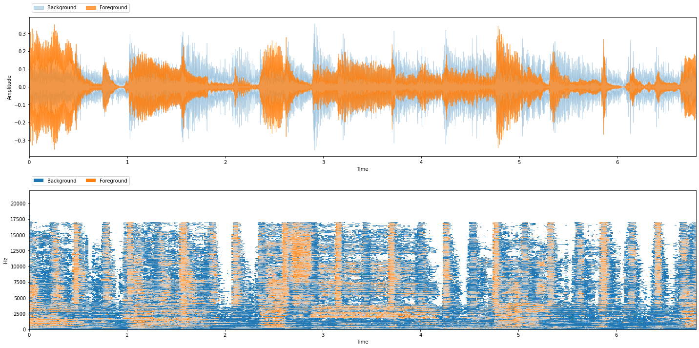
We can also use a Two-dimensional Fourier Transform (2DFT) of a spectrogram to find repeating and non-repeating patterns. [SPP17] Repeating sections show up as peaks in the 2DFT and non-repeating parts are everything else. We can use a peak picker to separate the repeating from non repeating parts. That’s what this algorithm does:

# We can't start a variable name with a number,
# so this object is called FT2D
ft2d = nussl.separation.primitive.FT2D(mix)
ft2d_bg, ft2d_fg = ft2d()

viz.show_sources({'Background': ft2d_bg, 'Foreground': ft2d_fg})

Let’s look at 2DFT’s evaluation metrics:

bss_eval = nussl.evaluation.BSSEvalScale(
    true_sources_list=[gt_bg, gt_fg],
    estimated_sources_list=[ft2d_bg, ft2d_fg]
)
ft2d_eval = bss_eval.evaluate()
print_metrics(ft2d_eval)

foreground SI-SDR: +1.50 dB
background SI-SDR: +7.46 dB

foreground SI-SAR: +3.45 dB
background SI-SAR: +8.83 dB

foreground SI-SIR: +6.11 dB
background SI-SIR: +13.15 dB

And let’s make 2DFT interactive too:

%%capture
# Comment out the line above to run this cell
# interactively in Colab or Jupyter Notebook

ft2d.interact(share=True, source='microphone')

Side-by-Side Comparison¶

Now that we have three repetition algorithms, let’s do a side-by-side comparison of them.

Let’s first look at the evaluation metrics of all three algorithms all at once:

print('REPET Metrics')
print('-------------')
print_metrics(repet_eval)
print('\n')

print('REPET-SIM Metrics')
print('-----------------')
print_metrics(rsim_eval)
print('\n')

print('2DFT Metrics')
print('------------')
print_metrics(ft2d_eval)

REPET Metrics
-------------
foreground SI-SDR: +1.95 dB
background SI-SDR: +7.29 dB

foreground SI-SAR: +3.85 dB
background SI-SAR: +7.79 dB

foreground SI-SIR: +6.66 dB
background SI-SIR: +16.88 dB



REPET-SIM Metrics
-----------------
foreground SI-SDR: +2.00 dB
background SI-SDR: +7.66 dB

foreground SI-SAR: +3.92 dB
background SI-SAR: +8.52 dB

foreground SI-SIR: +6.63 dB
background SI-SIR: +15.08 dB



2DFT Metrics
------------
foreground SI-SDR: +1.50 dB
background SI-SDR: +7.46 dB

foreground SI-SAR: +3.45 dB
background SI-SAR: +8.83 dB

foreground SI-SIR: +6.11 dB
background SI-SIR: +13.15 dB

Exercise¶

Spend some time playing with the interactive versions of REPET, REPET-SIM, and 2DFT. Which do you feel does best on the audio that you input? Do you feel that these evaluation metrics match your perception of each algorithm’s quality.