Representing Audio
The first thing we want to examine are the input and output representations of a source separation system and how the inputs and outputs are represented. In its most unprocessed form, we assume that audio is stored as a waveform. Some source separation approaches operate on the waveform directly, although many require some preprocessing before separating sources. In this section, we will discuss the different types of input and output representations that are commonly used in source separation approaches.
We’ll first start talking about waveforms, arguably the most fundamental representation of audio, then we’ll talk about what types of things are useful when we represent audio for source separation before we move onto some common audio representations for source separation.
Waveforms
Fig. 6 A waveform shown at many different time scales. Each value is sampled at a uniform rate and quantized. Image used courtesy of Jan Van Balen (source).
A waveform is shorthand for a digitized audio signal, which is most similar to what the sound is like physically. For an acoustic sound, the air pressure of over time changes, and is recorded by a microphone, which converts the changes in air pressure to an electrical signal. The voltage of this signal is sampled at a regular time interval, quantized, and converted to a digital array in a computer. This digital array is what we call the waveform. Of course, this description glosses over a lot of details in the realm of physics, acoustics, and signal processing. What’s important to know is that a continuous-time signal is discretized in both time and amplitude. We say a signal is monophonic, or mono, if there is only one audio channel, i.e., this array has shape \(x \in \mathbb{R}^{t \times 1}\). We say a signal is stereophonic, or stereo, if the array has two channels, i.e., this array has shape \(x \in \mathbb{R}^{t \times 2}\).
Note
Audio signals with more than 2 channels have many applications (e.g. 5.1 surround sound), including applications for in separating sources. Approaches that input many audio channels for separation are typically refered to under the title of beamforming approaches. Beamforming is a related, but separate area of active research. As such, the work we are going to cover in this space is sometimes called Single Channel Source Separation.
An important aspect of the waveform is the sample rate, which describes how many measurements, or samples, happen per second and is measured in Hertz, or Hz1. For a signal with sample rate \(sr\), the maximum frequency that can be reliably represented is \(f_N=\frac{sr}{2}\), which is called the Nyquist frequency. For example, if a signal has a sample rate of 44.1 kHz, the highest possible frequency is 22.05 kHz.
Many deep learning-based source separation approaches will reduce the sample rate of their input signals (called downsampling) to reduce the computational load during training time. Downsampling removes high frequency information from a signal, which is seen as a necessary evil when prototyping models.
Note
All of the source separation approaches we will discuss assume that the sample rate between the training, validation, and testing data is the same. The assumptions that ensure the approaches work are violated if the sample rate is variable. For example, if a system expects a signal at 16 kHz, then all input audio should be resampled to 16 kHz before using it.
Desirable Properties of Representations
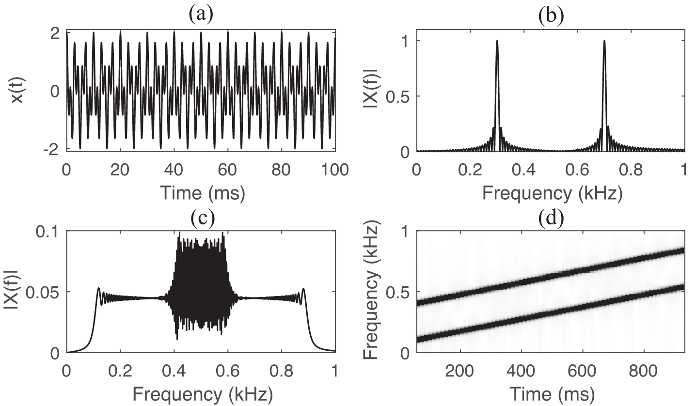
Fig. 7 Examples of two signals represented differently. The first row has two ways of displaying a mixture of two single-frequency sine waves; panel (a) represents the waveform and panel (b) shows the frequency spectrum. The second row has two ways of displaying a mixture of two linear chirp signals (i.e., sine waves with rising frequency); panel (c) shows a frequency spectrum and panel (d) shows a time-frequency representation. Notice how a signal that looks completely unseparable in one representation becomes easily separable in another representation. Image used courtesy of Fatemeh Pishdadian and Bryan Pardo. [PP18]
It can be argued that a source separation approach is only as good as its ability to represent audio in a separable manner. With that in mind, it’s important to understand how audio itself is represented for the purposes of source separation. For the source separation approaches we will explore here, we will see many variations on the same theme, namely:
Convert the audio to a representation easy to separate
Separate the audio by manipulating this representation
Convert the audio back from the manipulated representation to get isolated sources.
Almost every source separation approach we discuss here–classic and deep–can be broken down into these three steps. We want to note that each of these three steps might in fact involve multiple separate substeps.
Therefore an important aspect of an audio representation is invertability, or whether a signal that is converted from a waveform to a new representation can reliably be converted back to a waveform with little-to-no error. Artifacts that arise from converting back and forth will be audible in our separation output, so we want to minimize these types of errors (although eliminating them does not guarantee a perfect separation).
An other important aspect is whether this representation can keep data from one source apart from another source. As seen in Fig. 7, some representations might be better suited to separate certain signals than other representations. In this tutorial we will explore methods that produce representations specifically designed for separating sources.
Some recent source separations approaches use deep learning to learn a representation directly from the waveform, while others use preprocessing tools that are common in the audio signal processing and music information retrieval literature as a first step.
We will first discuss time frequency representations because they are an important preprocessing step, the parameters of which could have an impact on the separation quality of your approach.
Input Representations
Time-Frequency (TF) Representations
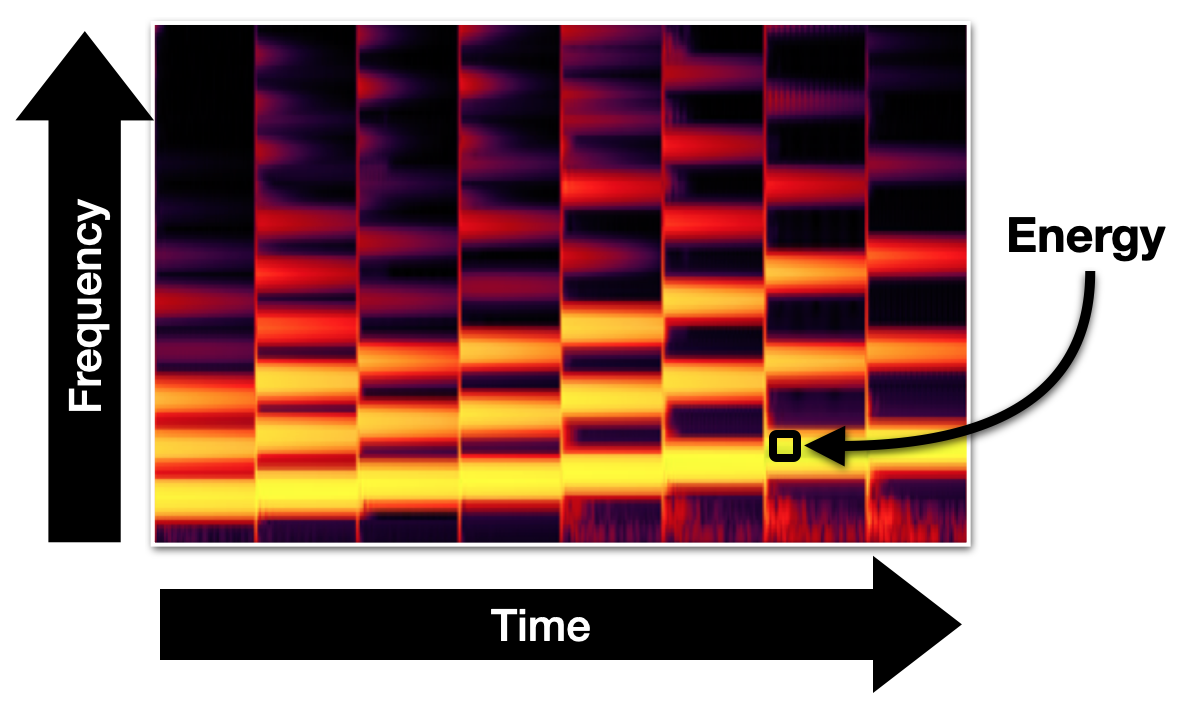
Fig. 8 A time-frequency representation. One dimension is indexed by time, another is index by frequency, and values in the matrix represent the energy of the sound at that partifular time and frequency.
A Time-Frequency [SI11] representation is a 2 dimensional matrix that represents the frequency contents of an audio signal over time. There are many types of time-frequency representations out in the world, but we will only discuss those that are most frequently used for source separation here.
We call a specific entry in this matrix a TF bin. We can visualize a TF Representation using a heatmap, which has time along the x-axis and frequency along the y-axis. Each TF bin in the heatmap represents the amplitude of the signal at that particular time and frequency. Some heatmaps have a colorbar alongside them that shows which colors indicate high amplitude values and which colors indicate low amplitude values. If there is no color bar, it is usually safe to assume that brighter colors indicate higher amplitudes than darker colors.
Time-frequency representations are the most common types of representations used in source separation approaches. Below we will outline some of the most popular and fundamental time-frequency representations.
Short-time Fourier Transform (STFT)
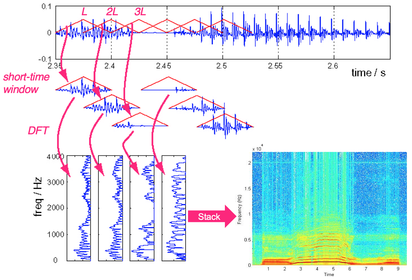
Fig. 9 The process of computing a short-time Fourier transform of a waveform. Imaged used courtesy of Bryan Pardo.
Many of the time-frequency representations that we will see in this tutorial start out as a Short-time Fourier Transform or STFT. An STFT is calculated from a waveform representation by computing a discrete Fourier transform (DFT) of a small, moving window2 across the duration of the window. The location of each entry in an STFT determines its time (x-axis) and frequency (y-axis). The absolute value of a TF bin \(|X(t, f)|\) at time \(t\) and frequency \(f\) determines the amount of energy heard from frequency \(f\) at time \(t\).
Importantly, each bin in our STFT is complex, meaning each entry contains both a magnitude component and a phase component. Both components are needed to convert an STFT matrix back to a waveform so that we may hear it.
The STFT is invertable, meaning that a complex valued STFT can be converted back to a waveform. This is called the inverse Short-time Fourier Transform or iSTFT.
Here are some important parameters to consider when computing an STFT:
Window Types
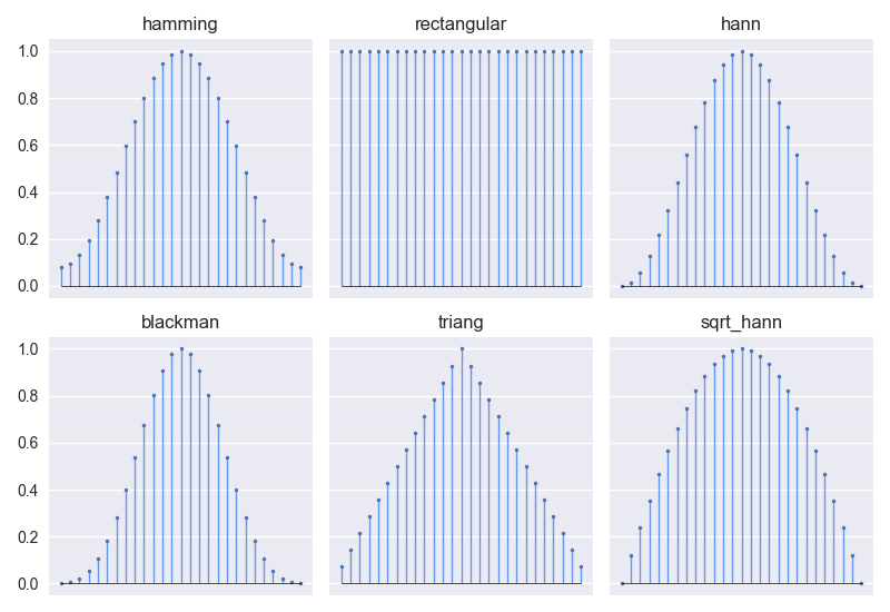
Fig. 10 Six commonly used window types for calculating an STFT.
The window type determines the shape of the short-time window that will segment
the audio into short segments before applying the DFT. The shape of this window
will affect which frequencies get emphasized or attenuated in the DFT. There
are many types of window functions, in Fig. 10, we show the most
common ones when calculating an STFT for source separation. For more information
on other types of windows and their frequency response, please see scipy.signal’s
documentation here.
Tip
We have informally noticed that our models acheive the best performance using
the sqrt_hann window, shown above.
Window Length
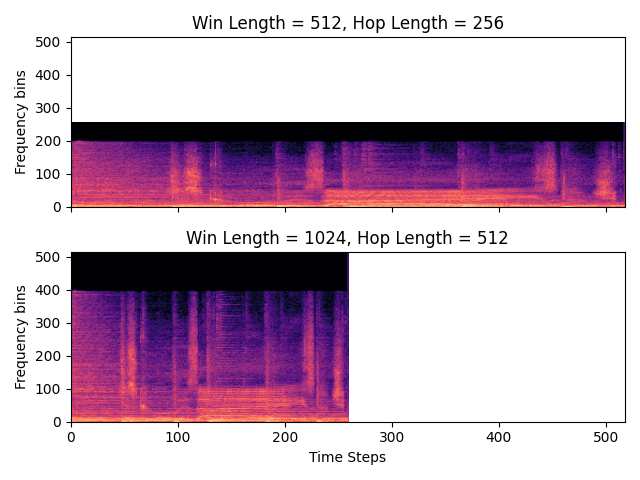
Fig. 11 Trade off between time and frequency resolution for different window lengths. In the simplified case, the number of frequency bins is determined by the window length. Using the same signal, we compute the STFT once with window length 512, and again with window length 1024. The white space is where there is no STFT data, which is left in to intentionally show how time and frequency interplay with the window length.
The window length determines how many samples are included in each short-time window. Due to how the DFT is computed, this parameter also determines the resolution of the frequency axis of the STFT. The longer the window, the higher the frequency resolution and vice versa, as is visible in Fig. 11.
Hop Length
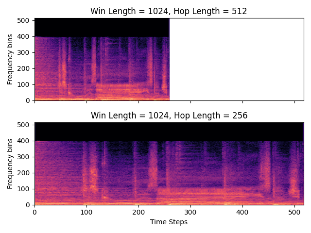
Fig. 12 The hop length determines the distance (in samples) between adjacent short-time windows. An STFT is computed twice on the same signal; the smaller the hop length the more times a particular segment of the audio signal is represented in the STFT.
The hop length determines the distance, in samples, between any two adjacent short-time windows. In the image shown in Fig. 12 shows how the hop length can elongate or shorten the time axis on an STFT depending on how it is set.
Overlap-Add
Many parameter settings for window type, window length, and hop length might not reconstruct the original signal perfectly when converting a signal to an STFT and back to a waveform. However, a certain set of parameters is mathematically guaranteed to perfectly reconstruct any signal. These parameter sets are called Constant Overlap-Add (COLA) because when applying successive windows, they add up to a constant value.
In general, we tend to use a hop length that is half of the window length, but there are many documented COLA settings, and an easy way to check if a tuple of settings is COLA.
Magnitude, Power, and Log Spectrograms
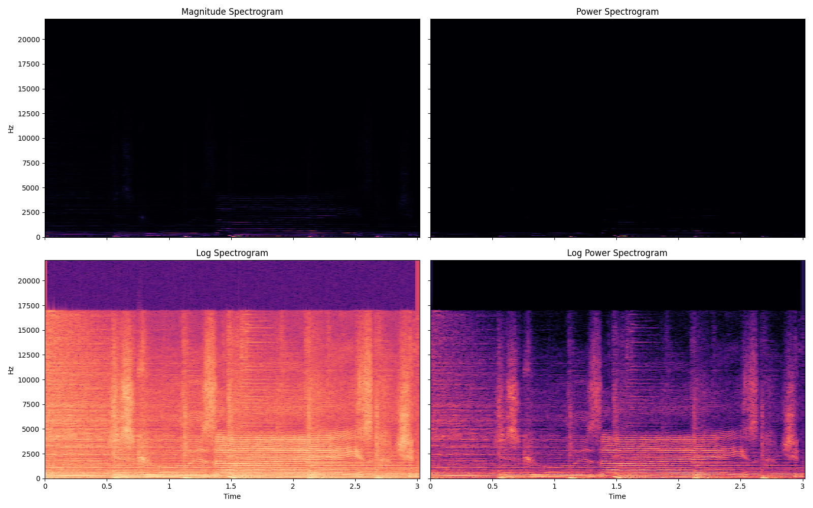
Fig. 13 A visual comparison of the four types of spectrograms discussed in this section. Each has a different scaling function applied to the loudness, which is reflected in the colors of the heatmap plots.
As we will touch on later in this tutorial, it is hard to model the phase of a signal. Therefore most source separation approaches only operate on the some variant of the spectrogram that does not explicitly represent phase in each TF bin. A visualization of four types of spectrograms is shown in Fig. 13.
Magnitude Spectrogram For a complex-valued STFT, \(X \in \mathbb{C}^{T \times F}\), the Magnitude Spectrogram is calculated by taking the absolute value of each element in the STFT, \(|X| \in \mathbb{R}^{T \times F}\).
Power Spectrogram For a complex-valued STFT, \(X \in \mathbb{C}^{T \times F}\), the Power Spectrogram is calculated by squaring each element in the STFT, \(|X|^2 \in \mathbb{R}^{T \times F}\).
Log Spectrogram Human hearing is logarithmic with regards to amplitude. For a complex-valued STFT, \(X \in \mathbb{C}^{T \times F}\), the Log Spectrogram is calculated taking the log of the absolute value of each element in the STFT, \(\log{|X|} \in \mathbb{R}^{T \times F}\).
Log Power Spectrogram For a complex-valued STFT, \(X \in \mathbb{C}^{T \times F}\), the Log Spectrogram is calculated taking the log of the square of each element in the STFT, \(\log{|X|^2} \in \mathbb{R}^{T \times F}\).
Tip
Even though it is hard to visualize the detail in a magnitude or power spectrogram, some source separation algorithms work completely fine on these representations, while some need log spectrograms. Make sure to set your spectrograms correctly!
Note
A note on terminology: while researchers might loosely interchange “STFT” and “spectrogram”, the term “spectrogram” is mostly used to describe a TF Representation that does not have any explicit phase representation. As such “spectrogram” might refer to a Magnitude Spectrogram, Power Spectrogram, Log Spectrogram, Mel Spectrogram, Log Mel Spectrogram, or similar. Use context clues to determine which representation is being discussed when possible.
Mel-spaced Spectrograms
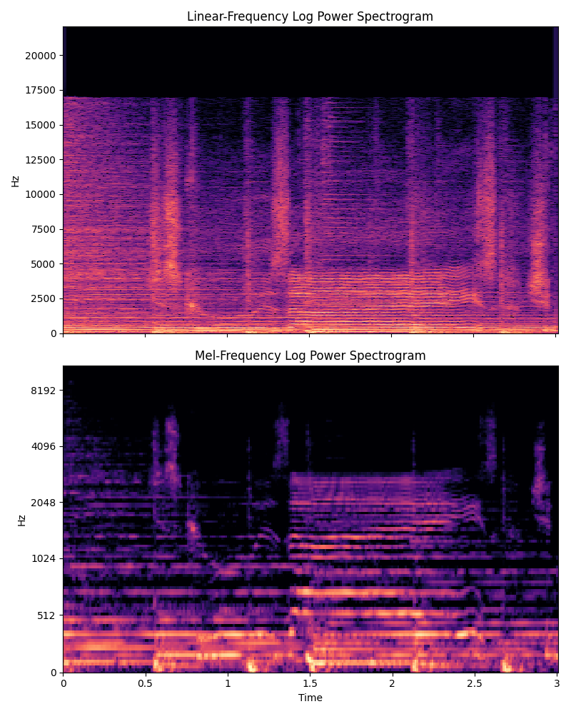
Fig. 14 A visual comparison of linear-scaled vs mel-spaced y axies. Lower frequencies have a larger representation in a mel-spaced spectrogram.
Human hearing is also logarithmic with regards to frequencies. The Mel scale approximates this property and is a quick way to make the frequency axis of a spectrogram quasi-logarithmic3. This is also commonly used to reduce the computational load on deep learning-based approaches, because the number of Mel-spaced frequency bins is often lower then the number of linearly-spaced frequency bins.
A visual comparison is shown in Fig. 14. Notice the how the y-axis in the Mel-spaced spectrogram is quasi-logarithmic, squishing higher frequencies and leaving more space for lower frequencies.
Other Representations
A few other representations have been explored in the literature. We provide references for a few below:
Constant-Q Transform (CQT)
Common Fate Transform (CFT) [StoterLB+16]
Multi-resolution Common Fate Transform (MCFT) [PP18]
2-Dimensional Fourier Transform (2DFT) [SPP17]
Per Channel Energy Normalization (PCEN) [LSC+18]
Output Representations
Ultimately, all source separation algorithms must be able to convert the audio that they processed back to a waveform. While some algorithms output waveforms directly, many algorithms output masks, which will be covered in more detail in the next sections. The masks get applied to the original mixture spectrogram, and that result is converted back to a waveform.
One thing to note is that if I have a waveform estimate for Source \(i\) from my mixture, then it is easy to calculate what the mixture sounds like without Source \(i\) present. Simply element-wise subtract the source waveform from the mixture waveform.
Which is Better? Inputting a Waveform or a Time-Frequency Representation?
Very few non-deep learning source separation approaches operate directly on waveforms, so we will restrict our answer to deep learning methods, which have dominated the field for the past few years. Even still, the answer is that it depends!
While this may change in the coming years, in general, determining which approach is best a very hard problem, as we will see in the Evaluation section.
In recent years, many state-of-the-art systems for music separation have used both spectrogram and waveforms as input. However, research in speech separation has mostly converged upon using the waveform as input. This may be a sign of things to come for music separation; we’ll have to wait and see!
By the end of this tutorial, we hope that you will be able to make an educated decision about which type of source system is right for your goals.
- 1
Named after Heinrich Hertz, who proved the existence of electromagnetic waves.
- 2
This window is where the term “Short-time” comes from in the name “Short-time Fourier Transform”.
- 3
librosa, arguably the most commonly used python library for MIR work, has two ways to convert from Hz to Mel, which are slightly different: see here.