Evaluation¶

Measuring the results of a source separation approach is a challenging problem. Generally, there are two main categories for evaluating the outputs of a source separation approach: objective and subjective. Objective measures rate separation quality by performing a set of calculations that compare the output signals of a separation system to the ground truth isolated sources. Subjective measures involve having human raters give scores for the source separation system’s output.

Objective and subjective measures both have benefits and drawbacks. Objective measures struggle because there are many aspects of human perception that are extremely difficult capture by computational means alone. However, compared to subjective measures, they are much faster and cheaper to obtain. On the other hand, subjective measures are expensive, time-consuming, and subject to the variability of human raters, but they can be more reliable than objective measures because actual human listeners are involved in the evaluation process.

Objective measures are, by far, much more popular than subjective measures, but we feel it is worth understanding them both to some extent.

Objective Measures¶

SDR, SIR, and SAR¶

Source-to-Distortion Ratio (SDR), Source-to-Interference Ratio (SIR), and Source-to-Artifact Ratio (SAR) are, to date, the most widely used methods for evaluating a source separation system’s output.

An estimate of a Source $\hat{s}_i$ is assumed to actually be composed of four separate components,

\[ \hat{s}_i = s_{\text{target}} + e_{\text{interf}} + e_{\text{noise}} + e_{\text{artif}}, \]

where $s_{\text{target}}$ is the true source, and $e_{\text{interf}}$, $e_{\text{noise}}$, and $e_{\text{artif}}$ are error terms for interference, noise, and added \text{artif}acts, respectively. The actual calculations of these terms is quite complex, so we refer the curious reader to the original paper for their exact calculation: [VGFevotte06].

Using these four terms, we can define our measures. All of the measures are in terms of decibels (dB), with higher values being better. To calculate they require access to the ground truth isolated sources and are usually calculated on a signal that has been divided into short windows of a few seconds long.

Source-to-Artifact Ratio (SAR)

\[ \text{SAR} := 10 \log_{10} \left( \frac{\| s_{\text{target}} + e_{\text{interf}} + e_{\text{noise}} \|^2}{ \| e_{\text{artif}} \|^2} \right) \]

This is usually interpreted as the amount of unwanted artifacts a source estimate has with relation to the true source.

Source-to-Interference Ratio (SIR)

\[ \text{SIR} := 10 \log_{10} \left( \frac{\| s_{\text{target}} \|^2}{ \| e_{\text{interf}} \|^2} \right) \]

This is usually interpreted as the amount of other sources that can be heard in a source estimate. This is most close to the concept of “bleed”, or “leakage”.

Source-to-Distortion Ratio (SDR)

\[ \text{SDR} := 10 \log_{10} \left( \frac{\| s_{\text{target}} \|^2}{ \| e_{\text{interf}} + e_{\text{noise}} + e_{\text{artif}} \|^2} \right) \]

SDR is usually considered to be an overall measure of how good a source sounds. If a paper only reports one number for estimated quality, it is usually SDR.

Note

As of this writing (October 2020), the best reported SDR for singing voice separation on MUSDB18 is $7.24 dB$. [TM20] Recent research papers have been reporting vocal SDRs on MUSDB18 in the range of 6-7 dB. Compare the SDR of different systems at this Papers with Code link.

Signal-to-Noise Ratio (SNR)

This is not used as widely, but does appear sometimes in source separation:

\[ \text{SNR} := 10 \log_{10} \left( \frac{\| s_{\text{target}} \|^2}{ \| s_{\text{target}} - \hat{s} \|^2} \right) \]

where $\hat{s}$ is the estimate of $s_{\text{target}}$.

SI-SDR¶

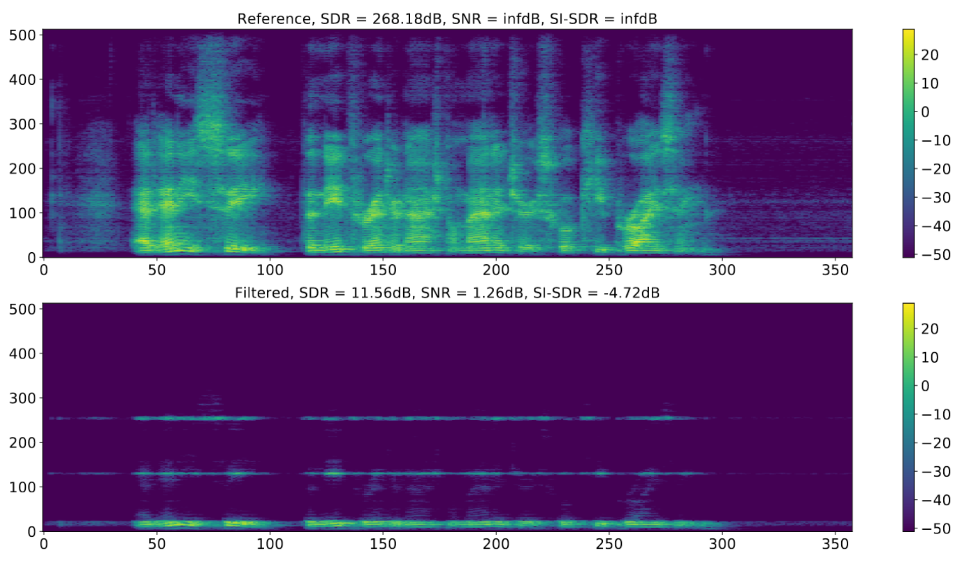
Waveform shown at many different time scales from a few seconds to a few samples.

Fig. 19 The way SDR calculates the $e_{\text{interf}}$, $e_{\text{noise}}$, and $e_{\text{artif}}$ terms can lead to issues where the original signal (top) can be horribly degraded (bottom) and still get a very high SDR score. Image used courtesy of Jonathan Le Roux. [LRWEH19]¶

A handful of issues have been brought up in the years since it was originally proposed. Although some of the issues are implementation-specific, one issue that persists is that SDR is easy to “cheat” on. The way that SDR calculates the $e_{\text{interf}}$, $e_{\text{noise}}$, and $e_{\text{artif}}$ terms can cause issues where scores are artificially inflated.

Scale-Invariant Source-to-Distortion Ratio (SI-SDR) aims to remedy this by removing SDR’s dependency on the amplitude scaling of the signal. [LRWEH19] It also comes with accompanying SI-SAR, and SI-SIR, which corresponds to SAR and SIR described above, respectively. Although these measures are not sensitive to amplitude scaling, it is a quicker computation because it does not require windowing the estimated and ground truth signals like SDR.

In Fig. 19, the discrepancy between SDR and SI-SDR scores is shown. The top spectrogram shows the ground truth signal. Above it are its scores for SDR, SNR, and SI-SDR. As expected the ground truth signal gets high values for SDR, SNR, and SI-SDR (268.1 dB, infinity dB, and infinity dB, respectively. Shown above the plot). The bottom spectrogram shows a highly degraded version of the top signal. While the SI-SDR, and SNR are quite low (-4.72 dB and 1.26 dB, respectively), the SDR value is still quite high (11.56 db). For reference, this is a speech signal and this SDR value is higher than state-of-the-art speech separation systems from a few years ago.

Reported SDRs¶

Many times SDRs are reported in research papers. When this happens, it is common to show just one number for SDR, but usually this number represents the mean of a distribution of SDRs calculated on a dataset. This is not the best practice, unfortunately, and the authors of this tutorial are certainly guilty of it. But when reading papers, be aware that this number is a summary statistic that could obscure a whole distribution.

Does Higher SDR Imply Better Quality?¶

SDR doesn’t tell you the whole story. Consider the following four audio examples. First is the input mixture, then the ground truth reference source, followed by two outputs from two different source separation models named ConvTasnet and Open-Unmix, respectively. Have a listen:

%%capture
!pip install nussl

Mixture

Reference Source

ConvTasnet Source

Open-Unmix Estimate

To our ears, the ConvTasnet output sounds much worse than the Open-Unmix output, but these two estimates both have the same SDR!

This is all to say that while SDR can give you a rough idea of how good an estimate might sound, it does not capture everything. Listen to your outputs!

(The original input mix and reference are from MUSDB18 and the separation examples kindly provided by Fabian-Robert Stöter.)

Subjective Measures¶

Having a human or set of humans evaluate a separation result is the gold standard for measuring the quality of a system. However, this is rarely done due to how difficult it is to get reliable evaluation data.

In a perfect world we would have a handful of well-trained audio engineers rate an algorithm’s output in a sound treated room. That’s exactly the formula for the MUSHRA tests, which rarely—if ever—happen when evaluating source separation because of how time-consuming and expensive they are.

Some studies have come have shown that crowd sourcing results from MUSHRA-like online listening studies can be an effective alternative to trained experts in a controlled setting. [CPMH16,SBStoter+18] Although this is much cheaper than a full-blown MUSHRA study, it still costs money ($100-200 USD) and takes a few days to get the results. Calculating SDR values on the other hand is virtually free and takes a few hours at most.

Open-Source Tools & Data for Music Source Separation