TF Representations and Masking
Masking has many uses in different aspects computer science and machine learning like language modelling and computer vision. It is also an essential part of how many modern source separation approaches approximate sources from a mixture. To separate a single source, a separation approach must create a single mask. To separate multiple sources, a separation approach must create multiple masks.
Masks are most commonly used with approaches that process a TF Representation, however you could make the case that some waveform-based deep learning architectures use masking within specific parts of their network (for instance see these papers: [LM18,LM19]). The content in this section, however, applies specifically to masking TF Representations.
For reasons we will fully discuss in the next section, we only apply masks to the magnitude values of a TF Representation, i.e., we do no apply masks to the phase component of an STFT. Because of this, in this section we will focus on masks applied to a spectrogram, where phase information is not explicitly represented.
What is a Mask?
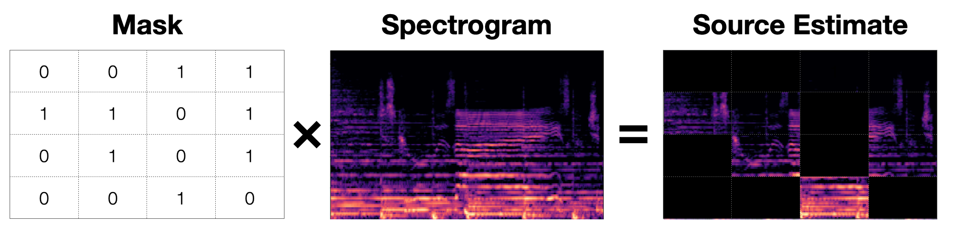
Fig. 15 A mask is a matrix with the same shape as the spectogram that is element-wise multiplied to it to produce a source estimate. This image shows an exaggerated binary mask that produces a source estimate. This estimate probably isn’t very good. ¯\_(ツ)_/¯
A mask is a matrix that is the same size as a spectrogram and contains values in the inclusive interval \([0.0, 1.0]\) 1. Each value in the mask determines what proportion of energy of the original mixture that a source contributes. In other words, for a particular TF bin, a value of \(1.0\) will allow all of the sound from the mixture through and a value of \(0.0\) will allow none of the sound from the mixture through.
We apply a mask to the original mixture by element-wise multiplying (sometimes called the Hadamard product2) the mask to the spectrogram. So if a mask, \(\hat{M}_i \in [0.0, 1.0]^{T \times F}\), represents the \(i\)th source, \(S_i\), in a mixture represented by a magnitude spectrogram, \(|Y| \in \mathbb{R}^{T \times F}\), we can make an estimate of the source like so:
We therefore hope that the mask we estimate \(\hat{M}_i\) is such that it can produce a good estimate of source \(S_i\) when we apply it.
For a mixture with \(N\) sources, the element-wise sum of every mask should equal a matrix of all ones, \(J \in [1.0]^{T \times F}\), that has the same shape as the masks (and spectrogram):
All this means is that combining all of our masks produces a matrix of all ones, which when we apply to the mixture, produces the original mixture (i.e. it does nothing because \(1 \times a = a\)).
This also means that we can remove Source \(i\) from the mix by “inverting” its mask, \(\hat{M}_i\). By “invert” here, we do not mean inverting the matrix in the traditional linear algebraic sense, but rather inverting every element individually, i.e., \(J - \hat{M}_i\). For example, if a value for Source \(i\) in \(\hat{M}_i\) is \(0.3\), the value of the mask for the rest of the mix at the corresponding bin is \(0.7\).
Binary Masks
The first mask type we’ll talk about is Binary Masks. Although not used much anymore, they can give us a good intuition about how masks work in practice.
As the name implies, Binary Masks are masks where the only values the entries are allowed to take is \(0.0\) or \(1.0\). Because all of the masks for the mixture element-wise sum up to a matrix of ones, a Binary Mask, therefore, makes the assumption that any TF bin is only dominated by exactly one source in the mixture. In the literature, this assumption is called W-disjoint orthogonality.
While Binary Masks are not used as much to produce final source estimates anymore, they are still useful as training targets, especially with neural network models like Deep Clustering, which we will discuss later in this tutorial.
Soft Masks (or Ratio Masks)
Soft Masks are allowed to take any value within the inclusive interval \([0.0, 1.0]\), which means that instead of assigning all of the energy from the mix to a source, it only assigns part of the mix’s energy to a source. This means that the energy in a mix from a TF bin can be split between the sources.
Soft masks are more flexible than binary masks and usually lead to better sounding results; it’s not very often that all of the energy in a mixture can always be assigned to one source.
Ideal Masks
As the name implies, an Ideal Mask, or Oracle Mask, represents the best possible performance for a mask-based source separation approach. Access to the ground truth isolated source is required in order to calculate an Ideal Mask mask for that source. As such, it is usually used as an upper limit on how well a source separation approach can do. Some recent waveform-based approaches for speech separation have surpassed the performance of Ideal Masks [LM19].
Next Steps
Assuming we have a mask for our signal that we’re happy with and we’ve applied it to our mixture signal to get an estimated magnitude spectrogram for our source, we still have the problem of turning the estimated source magnitude spectrogram back into audio so that we can listen to it. For that, we’ll need to understand phase, which we will discuss in the next section…
- 1
When we mix waves together, it is possible that the result is the product of constructive or destructive interference. Masking as we’ve presented it here does not account for either of these phenomena, although we do note that we are aware of some research papers [LRWW+19,CKH+18] that specifically designs for interference.
- 2
The element-wise product is notated a few different ways in the literature. For clarity, we use \(A \odot B\) here, but we have also seen it expressed as \(A \times B\) or \(A \cdot B\) for some matrices \(A\) and \(B\).