The MUSDB18 dataset
Overview
The information in this sub-section is based on the MUSB18 dataset page. [RLStoter+17,RLS+19] Here we have edited down the content to focus on the details relevant to this tutorial while keeping it concise. For more details about the datataset please consult the dataset page.
MUSDB18 is a dataset of 150 full length music tracks (~10h total duration) of varying genres. For each track it provides:
The mixture
And the following stems:
Drums
Bass
Vocals
Other
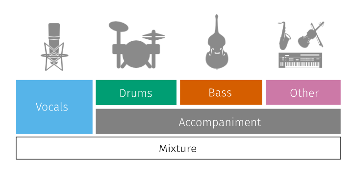
As its name suggests, the “other” stem contains all other sources in the mix that are not the drums, bass or vocals (labeled as “accompaniment” in the diagram below):

Fig. 46 Illustration of the stems comprising the mixture in a MUSDB18 track. Source: https://sigsep.github.io/.
All audio signals in the dataset are stereo and encoded at a sampling rate of 44.1 kHz. The mixture signal is identical to the sum of the stems.
The data in MUSDB18 is compiled from multiple sources: the DSD100 dataset, the MedleyDB dataset, the Native Instruments stems pack, and the The Easton Ellises - heise stems remix competition.
Note
MUSDB18 can be used for academic purposes only, with multiple of its tracks licensed under a Creative Commons Non-Commercial Share Alike license (BY-NC-SA).
The full dataset is divided into train and test folders with 100 and 50 songs respectively. As their names suggest, the former should be used for model training and the latter for model evaluation.
Note
You do not need to download the full MUSDB18 dataset to complete this tutorial. For simplicity, we’ll be using short excerpts (clips) from this dataset which
we will download via the nussl python library in the next step.
The dataset was created by Zafar Rafii, Antoine Liutkus, Fabian-Robert Stöter, Stylianos Ioannis Mimilakis, and Rachel Bittner. When using the dataset in your work, please be sure to cite it as:
@misc{musdb18,
author = {Rafii, Zafar and
Liutkus, Antoine and
Fabian-Robert St{\"o}ter and
Mimilakis, Stylianos Ioannis and
Bittner, Rachel},
title = {The {MUSDB18} corpus for music separation},
month = dec,
year = 2017,
doi = {10.5281/zenodo.1117372},
url = {https://doi.org/10.5281/zenodo.1117372}
}
Downloading and inspecting MUSDB18 clips
Downloading MUSDB18 clips with nussl
We’ll use nussl, the source separation library used in this tutorial, to download 7-second clips from MUSDB18. We’ll get into nussl in greater detail in the next Chapter, but for we’ll just use it to download and inspect the audio clips.
Let’s start by installing nussl. We’ll also install a package we wrote especially for this tutorial, common, that will help us visualize data easily.
%%capture
!pip install nussl
!pip install git+https://github.com/source-separation/tutorial
Now we’re ready to import the tools we need for this section:
import nussl
from IPython.display import Audio
import IPython
from common import viz
The following cell will download 7-second clips for 143 of the 150 tracks in the dataset (the remaining 7 tracks do not have preview clips due to copyright, but are included in the full dataset):
# Run this command to download X 7-second clips from MUSDB18
musdb = nussl.datasets.MUSDB18(download=True)
Once the dataset has been downloaded to disk, subsequent instantiations of the MUSDB18 class will skip the download step.
Inspecting MUSDB18 clips
Let’s get the just training data:
musdb_train = nussl.datasets.MUSDB18(subsets=['train'])
print(musdb_train.items)
[0, 1, 2, 3, 4, 5, 6, 7, 8, 9, 10, 11, 12, 13, 14, 15, 16, 17, 18, 19, 20, 21, 22, 23, 24, 25, 26, 27, 28, 29, 30, 31, 32, 33, 34, 35, 36, 37, 38, 39, 40, 41, 42, 43, 44, 45, 46, 47, 48, 49, 50, 51, 52, 53, 54, 55, 56, 57, 58, 59, 60, 61, 62, 63, 64, 65, 66, 67, 68, 69, 70, 71, 72, 73, 74, 75, 76, 77, 78, 79, 80, 81, 82, 83, 84, 85, 86, 87, 88, 89, 90, 91, 92, 93]
We see there are 94 tracks in the train set. Let’s explore the first item:
idx = 0
item = musdb_train[idx]
item.keys()
dict_keys(['mix', 'sources', 'metadata'])
Each item is a dictionary containing the mix, sources (stems), and metadata. The metadata for this item includes a list of stem labels:
item['metadata']
{'labels': ['bass', 'drums', 'other', 'vocals']}
We can also get this list by print the keys of the sources dictoinary:
item['sources'].keys()
dict_keys(['drums', 'bass', 'other', 'vocals'])
Let’s listen to the mix:
Audio(data=item['mix'].audio_data, rate=item['mix'].sample_rate)
Now let’s listen to each stem:
for stem_label in item['sources'].keys():
print(stem_label)
audio_player = Audio(data=item['sources'][stem_label].audio_data, rate=item['sources'][stem_label].sample_rate)
IPython.display.display(audio_player)
drums
bass
other
vocals
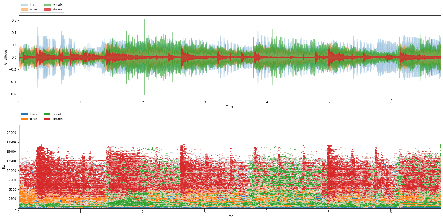
Now let’s plot the audio data. We could do this via matplotlib or librosa, but to make life easy, for this tutorial we’ve create a viz module which provides a show_sources function which:
Takes a dictionary of stems (sources) as input
Plots the audio signal of each stems in a different color, all in one subplot
Plots the stems as time-frequency masks (more on this later) in a second subplot
Creates an audio player where you can play all the stems together or selectively mute/solo each stem:
viz.show_sources(item['sources'])

Exercise
Repeat the above steps for several items in the train set. What can you tell about the data from listening to it?
Exercise
Repeat the above steps for several items from the test set, and answer:
Do the train and test sets contain the same instruments?
Is the train set representative of the musical data in the test set?
Do you expect a model trained on the train set to generalize well to the test set?
Great, now that we’ve download and explored our data, we are ready to learn how to use Scaper to generate augmented training mixtures on the fly.